Multivariate TS Models(ARIMAX/SARIMAX/VAR)

Author

zoo un park

note

Currently there are four models, but more models will be added

This project examines how U.S. economic and financial conditions transmit to South Korea’s economy across markets and the real sector. Because there are many candidate indicators—spanning growth, risk sentiment, interest rates, exchange rates, and trade—careful variable selection is essential before modeling. Goal of this section is to build multivariate models to answer four questions:

1. how U.S. and Korean equities interact
1. how the Seoul metropolitan housing market responds to Long end of the term structure
1. which exogenous factors move the won–dollar exchange rate
1. which factors drive Korea’s exports to the U.S.

Literature reviews

Before turning to the analysis, a targeted literature review aligns the four questions with the overarching research objective and justifies each modeling choice.

In U.S.–South Korea equity linkages, Kim (2010)¹ documents significant spillovers in higher moments (mean, volatility, skewness, kurtosis) between U.S. and Korean equity markets using high-frequency data, indicating that U.S. shocks propagate to Korean returns; more recently, a study in Business and Economic Research shows that changes in the VIX are negatively associated with KOSPI returns, reinforcing a U.S. risk-to-Korea transmission channel. Together, these results support a VAR that treats U.S. equity performance and global risk as upstream drivers of Korean equities, with a discount-rate control: include Δlog(S&P 500), VIX, Δlog(KOSPI), and a U.S. yield spread (10Y–3M or 10Y–2Y) to capture the rate channel affecting both markets.

For the Seoul housing market, Lee (2022)² uses a Korean time-varying parameter VAR (1991–2022) and finds that the impact of interest-rate shocks on housing prices strengthened markedly after the global financial crisis, implying state-dependent pass-through from rates to valuations. Complementary evidence from Min (2024)³ likewise highlights time-varying impulse responses of Seoul housing to interest rates. These findings motivate a compact VAR comprising the U.S. 10-year Treasury yield, the Korea 10-year government bond yield, and the log of the Seoul housing price index, ordered to trace global-to-local rate pass-through and then housing, while leaving room to test time variation via rolling windows or TVP extensions.

For the KRW/USD exchange rate, Yoon (2019)⁴ argues that U.S. monetary conditions dominate KRW/USD dynamics given the dollar-centric trading of Korea’s FX market, while Masujima (2018, RIETI)⁵ adds that exchange-rate drivers rotate across carry (rate differentials), the global dollar factor, and risk sentiment (VIX). These insights support a SARIMAX for Δlog(USD/KRW) with exogenous terms for the U.S.–Korea interest-rate spread (3Y or 10Y), Δlog(Dollar Index, DXY) to capture the global dollar cycle, and a risk proxy (VIX or Δlog(S&P 500))—a structure also consistent with funding-risk episodes highlighted for Korea by the IMF.

Finally, on South Korea’s exports to the United States, a Bank of Korea working paper on dominant currency pricing (Son et al., 2023)⁶ shows that Korean exports are heavily invoiced in U.S. dollars due to strategic complementarities and real hedging, implying that the dollar level often matters for short-run trade revenues. Pairing this with a U.S. demand proxy captures the real-side pull. Accordingly, model Δlog(Korea’s exports to the United States) with U.S. manufacturing demand (ISM Manufacturing PMI or U.S. industrial production), an exchange-rate term (Δlog(USD/KRW) and/or DXY for invoicing effects), and a risk/financing control (VIX), with seasonal terms for monthly data.

Code

library(tidyverse)
library(ggplot2)
library(forecast)
library(astsa) 
library(xts)
library(zoo)
library(tseries)
library(fpp2)
library(fma)
library(lubridate)
library(tidyverse)
library(TSstudio)
library(tidyquant)
library(plotly)
library(readr)
library(kableExtra)
library(knitr)
library(patchwork)
library(vars)
library(here)
library(tsibble)
library(dplyr)
# calling data

#KR base rate
bok<- read.csv("../data/interest/bok.csv")%>%
  rename(Date = date)
bok$Date<- as.Date(bok$Date)
bok <- bok %>%
  mutate(Date = floor_date(Date, unit = "quarter")) %>%
  group_by(Date) %>%
  summarise(across(where(is.numeric), ~ mean(.x, na.rm = TRUE)), .groups = "drop")


# FED rate 

usr<- read.csv("../data/interest/us_rate.csv")%>%
  rename(Date = observation_date,rate = DFF)
usr$Date<- as.Date(usr$Date)
usr<- usr %>%
  mutate(Date = floor_date(Date, unit = "quarter")) %>%
  group_by(Date) %>%
  summarise(across(where(is.numeric), ~ mean(.x, na.rm = TRUE)), .groups = "drop")

# KRW/USD rate

kr <- read.csv("../data/fx rate/kor.csv")
kr <- kr %>%
  transmute(
    Date = as.Date(observation_date),
    krw  = DEXKOUS,    
    usd  = 1 / DEXKOUS  
  ) %>%
  filter(!is.na(Date)) %>%
  arrange(Date) %>%
  distinct(Date, .keep_all = TRUE) %>%
  complete(Date = seq(min(Date), max(Date), by = "day")) %>%

  fill(krw, usd, .direction = "down")


# USD index 

usd <- read_csv("../data/fx rate/usd_index.csv", show_col_types = FALSE)
usd <- usd %>%
  transmute(
    Date = as.Date(Date),
    usd_index = Close
  ) %>%
  filter(!is.na(Date)) %>%
  arrange(Date) %>%
  distinct(Date, .keep_all = TRUE) %>%
  complete(Date = seq(min(Date), max(Date), by = "day")) %>%
  fill(usd_index, .direction = "down")



# Seoul housing data

housing <- read_csv(here("data/housing/house.csv")) %>%
  mutate(Date = as.Date(Date))

housing <- housing %>% mutate(Date = as.Date(Date))


# Yield data 

us_yield  <- read.csv(here("data/yield", "us_yield.csv"))
kor_yield   <- read.csv(here("data/yield", "kor_yield.csv"))


us_yield$Date  <- as.Date(us_yield$Date)
kor_yield$Date <- as.Date(kor_yield$Date)

colnames(us_yield)[colnames(us_yield)  == "X3Y"]  <- "US_3Y"
colnames(us_yield)[colnames(us_yield)  == "X10Y"] <- "US_10Y"
colnames(kor_yield)[colnames(kor_yield) == "X3Y"]  <- "KR_3Y"
colnames(kor_yield)[colnames(kor_yield) == "X10Y"] <- "KR_10Y"

us_yield  <- us_yield[,  c("Date", "US_3Y", "US_10Y")]
kor_yield <- kor_yield[, c("Date", "KR_3Y", "KR_10Y")]

us_yield  <- us_yield  %>% arrange(Date) %>% fill(US_3Y, US_10Y, .direction = "down")
kor_yield <- kor_yield %>% arrange(Date) %>% fill(KR_3Y, KR_10Y, .direction = "down")


df <- merge(us_yield, kor_yield, by = "Date")

df$US_3m10  <- df$US_3Y - df$US_10Y
df$KR_3m10  <- df$KR_3Y - df$KR_10Y
df$US_KR_3Y <- df$US_3Y - df$KR_3Y
df$US_KR_10Y<- df$US_10Y - df$KR_10Y


#import & export data 

trade<- read_csv("../data/trade/trade_merged.csv")
trade$balance<- trade$export_USD - trade$import_USD
exports<- trade%>%
  dplyr::select(Date,export_USD)
#trade_ts <- trade %>%
 # as_tsibble(index = Date, key = Type)


# S&P500 data
sp500 <- read_csv("../data/stock/sp500.csv")


# KOSPI data
kospi <- read_csv("../data/stock/kospi.csv")
kospi$Date <- as.Date(kospi$Date)

# VIX data(added for the modeling)
vix<- read_csv("../data/stock/vix.csv")%>%
  mutate(Date = ymd(Date)) %>%
  arrange(Date) %>%
  fill(vix, .direction = "down")


# extract spreads from df


us_spreads <- df %>%
  dplyr::select(Date, US_3m10) %>%
  rename(us_spread = US_3m10) %>%
  mutate(Date = as.Date(Date))

kor_spreads <- df %>%
  dplyr::select(Date, KR_3m10) %>%
  rename(kr_spread = KR_3m10) %>%
  mutate(Date = as.Date(Date))

us_kr_spreads_3y <- df %>%
  dplyr::select(Date, US_KR_3Y) %>%
  mutate(Date = as.Date(Date))

us_kr_spreads_10y <- df %>%
  dplyr::select(Date, US_KR_10Y) %>%
  mutate(Date = as.Date(Date))

# balance of payment(debt,equity)

bp<- read_csv("../data/bp.csv")%>%
  mutate(Date = ymd(Date)) %>%
  rename(debt_securities = "Debt securities of P.I., Liabilities")%>%
  rename(equity_securities = "Equity securities of P.I., Liabilities")%>%
  arrange(Date)

bp_debt<- data.frame(bp$Date,bp$debt_securities)
bp_equity<- data.frame(bp$Date,bp$equity_securities)
bp_debt<- bp_debt%>%rename(Date = bp.Date, debt_securities= bp.debt_securities)
bp_equity<- bp_equity%>%rename(Date = bp.Date, equity_securities= bp.equity_securities)

#oil price 

oil<- read_csv("../data/oil.csv")%>%
  rename(Date = observation_date)%>%
  rename(wti = DCOILWTICO)%>%
  mutate(Date = ymd(Date)) %>%
  arrange(Date)%>%
  fill(wti, .direction = "down")

debt_monthly <- bp_debt %>%
  mutate(year_month = floor_date(Date, "month")) %>%
  group_by(year_month) %>%
  slice_tail(n = 1) %>%
  ungroup() %>%
  mutate(Date = ceiling_date(year_month, "month") - days(1))%>%
  dplyr::select(Date,debt_securities)

equity_monthly <- bp_equity %>%
  mutate(year_month = floor_date(Date, "month")) %>%
  group_by(year_month) %>%
  slice_tail(n = 1) %>%
  ungroup() %>%
  mutate(Date = ceiling_date(year_month, "month") - days(1))%>%
  dplyr::select(Date,equity_securities)


vix_monthly <- vix %>%
  mutate(year_month = floor_date(Date, "month")) %>%
  group_by(year_month) %>%
  slice_tail(n = 1) %>%
  ungroup() %>%
  mutate(Date = ceiling_date(year_month, "month") - days(1))%>%
  dplyr::select(Date,vix)

Variables

FX spot rate (KRW per USD)

The bilateral exchange rate quoted as won per dollar; it moves up when the USD strengthens or U.S. rates/risk rise and down when KRW demand or relative KR rates strengthen; up-moves mean a weaker KRW and costlier imports/funding while down-moves mean stronger KRW and easier external conditions; it matters because it transmits U.S. financial shifts into Korea’s prices, trade margins, and capital flows.

U.S.–Korea 3-year yield spread

The 3Y U.S. Treasury yield minus the 3Y Korea Treasury Bond yield; it widens when U.S. front-to-belly rates outpace Korea’s and narrows when Korea’s rise or U.S. fall; widening implies policy divergence favoring USD assets and KRW pressure, narrowing implies the opposite; it matters as a near-term compass for FX, flows, and local funding costs.

U.S.–Korea 10-year yield spread

The 10Y U.S. Treasury yield minus the 10Y Korea government bond yield; it moves with relative long-run growth/inflation expectations and term premium; wider spreads signal capital preference for U.S. duration and KRW headwinds, narrower spreads point to relatively easier conditions for Korea; it matters for portfolio allocations, currency valuation, and long-tenor financing.

S&P 500 index

The main U.S. large-capital equity benchmark; it rises with stronger earnings/risk appetite and falls on growth scares or tighter policy; gains signal global risk-on that often supports KOSPI and KRW, while declines flag risk-off and potential outflows from Korea; it matters as the world’s equity bellwether shaping cross-border sentiment.

Dollar Index (DXY)

A broad USD index versus major currencies(JPY,GBP,EUR,CAD,SEK,CHF); it rises with stronger U.S. growth/real yields or heightened risk and falls when global growth broadens or the Fed eases; increases mean tighter global financial conditions and KRW headwinds, decreases mean relief; it matters because it frames Korea’s external competitiveness and dollar funding costs.

South Korea exports to the United States (USD)

The monthly value of Korean goods shipped to the U.S.; it rises with firm U.S. demand/tech upcycles and falls when U.S. activity softens or conditions tighten; increases mean stronger external demand and earnings support for Korea, decreases warn of slower production and profits; it matters as a direct real-economy link between the two countries.

VIX (U.S. equity volatility index)

Implied 30-day volatility from S&P 500 options; it spikes in stress and recedes in calm; higher readings mean risk-off, likely KRW weakness and KOSPI pressure, lower readings mean risk-on support; it matters as a fast, forward-looking gauge of global risk that transmits into Korean assets.

U.S. manufacturing index (ISM Manufacturing PMI)

A diffusion index of U.S. factory activity where 50 marks expansion; it rises with stronger orders/production and falls with slowdowns; higher prints mean firmer U.S. goods demand that often lifts Korean exports, lower prints caution on future orders; it matters as a timely cue for Korea’s trade and industrial cycle.

U.S. yield spread (10Y–3Y curve slope)

The term spread between long and intermediate Treasuries; it steepens on improving growth/term premium and inverts ahead of slowdowns; steepening often signals risk-on and better global momentum, inversion warns of softer demand; it matters because it foreshadows the external environment Korea will face.

KOSPI index

Korea’s main equity benchmark; it rises with global risk appetite, stable/strong KRW, and tech strength, and falls when the dollar tightens conditions or volatility jumps; up-moves mean improving earnings/flows, down-moves mean de-risking and potential outflows; it matters as the market-price readout of Korea’s cyclical exposure to U.S. conditions.

U.S. 10-year Treasury yield

The anchor long-term U.S. risk-free rate; it rises on stronger growth/less-dovish policy or higher term premium and falls on easing or growth fears; higher yields mean tighter global discount rates and KRW/KOSPI headwinds, lower yields mean relief; it matters because it sets the tone for valuation and borrowing costs worldwide.

South Korea 10-year government bond yield

Korea’s benchmark long-term sovereign yield; it rises with domestic inflation/growth or spillovers from higher U.S. yields and falls with easing/disinflation; increases mean tighter local conditions and pricier mortgages/corporate debt, decreases mean looser conditions; it matters for domestic credit, housing, and investment.

Seoul residential property price index

An index of Seoul home prices; it rises with lower mortgage rates/strong incomes and softens when rates rise or credit tightens; up-moves signal wealth effects and consumption support, down-moves flag cooling demand and potential credit restraint; it matters as a slower-moving but powerful transmission channel from global rates to the household economy.

Model explanation

VAR model 1 — Equity co-movements (S&P 500, VIX, U.S. yield spread, KOSPI)

Financial linkages transmit U.S. equity and risk shocks to Korean equities through discount-rate and sentiment channels, with feedback over short horizons. The VAR includes Δlog(S&P 500), VIX, the U.S. yield spread (10Y–3M or 10Y–2Y), and Δlog(KOSPI) as jointly endogenous variables. This set captures the main transmission mechanisms: the yield spread summarizes shifts in discount rates and growth expectations; S&P 500 represents U.S. equity innovations; VIX captures global risk aversion; and KOSPI reflects Korea’s market response. A VAR is justified because these variables interact contemporaneously and with lags; the system enables impulse responses from U.S. rate/equity/risk shocks to KOSPI, and variance decompositions that quantify the U.S. contribution to Korean equity volatility.

VAR model 2 — Rates pass-through and Seoul housing (US10Y, KR10Y, Seoul HPI)

Housing valuations in Seoul are sensitive to financing conditions, and global rate movements typically filter through to domestic long-term yields before affecting prices with lags. The VAR comprises the U.S. 10-year Treasury yield, the Korea 10-year government bond yield, and the log of the Seoul housing price index. This configuration reflects a plausible ordering of influences: global long rates anchor international term structures, domestic long rates transmit the shock into local borrowing costs and mortgage pricing, and housing prices adjust gradually via affordability and discount-rate channels. A VAR is warranted because long rates and housing prices exhibit mutual dynamics and delayed pass-through; the framework traces how a U.S. term-structure shock propagates to Korean yields and then to housing over time, while allowing tests for lag length, stability, and time-variation.

SARIMAX model 1 — USD/KRW determinants

Exchange-rate behavior in Korea is strongly influenced by cross-border interest-rate differentials, global risk sentiment, and the broad dollar cycle, reflecting the market’s integration with U.S. monetary conditions and dollar funding. The model includes the U.S.–Korea 3-year yield spread, the S&P 500, and the Dollar Index (DXY) as exogenous drivers of USD/KRW. The spread captures carry/UIP forces and relative monetary stance; the S&P 500 serves as a high-frequency proxy for global risk-on/off that tends to strengthen or weaken KRW; and DXY isolates the common dollar factor that moves bilateral rates beyond country-specific fundamentals. SARIMAX fits because USD/KRW exhibits strong serial correlation that ARIMA errors can handle, while the exogenous block reflects reasonably weakly exogenous global forces at the chosen frequency.

SARIMAX model 2— South Korea exports to the U.S.

International trade research shows that partner-country demand, currency valuation, and global risk conditions jointly shape export dynamics—especially for economies like Korea that are tightly linked to U.S. manufacturing cycles and invoice a large share of exports in dollars. The model uses U.S. manufacturing activity (e.g., ISM Manufacturing PMI or U.S. industrial production), the KRW/USD spot rate, and the VIX as exogenous regressors for South Korea’s exports to the U.S. This selection is justified by clear channels: the U.S. manufacturing index captures external demand pull; the KRW/USD rate captures pricing and competitiveness as well as dollar-denominated revenue effects; and the VIX proxies global financial conditions that influence trade finance, inventory decisions, and risk-sensitive orders. A SARIMAX structure is appropriate because exports are persistent and seasonal, allowing ARIMA terms to absorb autocorrelation and seasonality while treating the U.S. indicators and VIX as upstream drivers at monthly frequency.

Models

SARIMAX:

South korea exports(vs USA) ~ VIX + US manufacturing Index + KRW/USD spot rate
USD/KRW spot rate ~ us-korea spread rate 3years+ us-korea spread rate 3years+ S&P500 + dollar index

VAR:

equity: s&p500, vix, us_yield_spread,KOSPI index
US treasury yield curve 10 Years, South Korea government bond rate 10Years, Seoul housing index

VAR model

equity: s&p500, us_yield_spread,KOSPI index

Code

library(dplyr)
df1 <- us_spreads %>%
   left_join(sp500, by = "Date") %>%
   left_join(kospi, by = "Date")%>%
   dplyr::select(Date, us_spread, close_sp500 = Close.x , close_kospi = Close.y)%>%
   arrange(Date) %>%
   fill(close_sp500,close_kospi, .direction = "down")
 
df1$log_kospi<- log(df1$close_kospi)
df1$log_sp500<- log(df1$close_sp500)


 start_year_df1  <- year(min(df1$Date))
 start_month_df1 <- month(min(df1$Date))


p1 <- plot_ly(df1, x = ~Date, y = ~us_spread, type = 'scatter', mode = 'lines',
              name = "U.S Spread Rate") %>%
  layout(yaxis = list(title = "U.S Spread Rate", titlefont = list(size = 14), tickfont = list(size = 12)))

p2 <- plot_ly(df1, x = ~Date, y = ~log_sp500, type = 'scatter', mode = 'lines',
              name = "S&P500 Index(log)") %>%
  layout(yaxis = list(title = "S&P500 Index(log)", titlefont = list(size = 14), tickfont = list(size = 12)))

p3 <- plot_ly(df1, x = ~Date, y = ~log_kospi, type = 'scatter', mode = 'lines',
              name = "KOSPI Index(log)") %>%
  layout(yaxis = list(title = "KOSPI Index(log)", titlefont = list(size = 14), tickfont = list(size = 12)))

subplot(p1, p2, p3, nrows = 3, shareX = TRUE, titleX = TRUE) %>%
  layout(title = list(text = "Equities:KOSPI index, S&P 500 index, U.S T-bond spread rate", font = list(size = 18)),
         margin = list(l = 70, r = 40, t = 60, b = 40))

Code

new_df1<- df1[,c(2,5,6)]
df1.ts<-ts(new_df1,star=decimal_date(as.Date("2001-12-01",format = "%Y-%m-%d")),frequency = 252)
VARselect(df1.ts, lag.max=10, type="both")

$selection
AIC(n)  HQ(n)  SC(n) FPE(n) 
    10      5      2     10 

$criteria
                   1             2             3             4             5
AIC(n) -2.419658e+01 -2.436948e+01 -2.437841e+01 -2.438541e+01 -2.438900e+01
HQ(n)  -2.419068e+01 -2.436005e+01 -2.436544e+01 -2.436890e+01 -2.436895e+01
SC(n)  -2.417962e+01 -2.434234e+01 -2.434109e+01 -2.433791e+01 -2.433132e+01
FPE(n)  3.101405e-11  2.608965e-11  2.585770e-11  2.567740e-11  2.558543e-11
                   6             7             8             9            10
AIC(n) -2.439247e+01 -2.439309e+01 -2.439656e+01 -2.440048e+01 -2.440168e+01
HQ(n)  -2.436889e+01 -2.436597e+01 -2.436590e+01 -2.436628e+01 -2.436394e+01
SC(n)  -2.432461e+01 -2.431505e+01 -2.430834e+01 -2.430208e+01 -2.429310e+01
FPE(n)  2.549667e-11  2.548083e-11  2.539261e-11  2.529342e-11  2.526311e-11

From parameter selction process, three parameters were suggested; p = 2,5,10

Code

summary(fit <- VAR(new_df1, p=2, type="both"))


VAR Estimation Results:
========================= 
Endogenous variables: us_spread, log_kospi, log_sp500 
Deterministic variables: both 
Sample size: 5918 
Log Likelihood: 46927.097 
Roots of the characteristic polynomial:
0.9987 0.9979 0.9954 0.2162 0.0273 0.0273
Call:
VAR(y = new_df1, p = 2, type = "both")


Estimation results for equation us_spread: 
========================================== 
us_spread = us_spread.l1 + log_kospi.l1 + log_sp500.l1 + us_spread.l2 + log_kospi.l2 + log_sp500.l2 + const + trend 

               Estimate Std. Error t value Pr(>|t|)    
us_spread.l1  1.005e+00  1.302e-02  77.209   <2e-16 ***
log_kospi.l1  4.318e-02  3.263e-02   1.324    0.186    
log_sp500.l1  5.690e-02  3.593e-02   1.583    0.113    
us_spread.l2 -7.440e-03  1.302e-02  -0.572    0.568    
log_kospi.l2 -4.234e-02  3.264e-02  -1.297    0.195    
log_sp500.l2 -5.388e-02  3.591e-02  -1.501    0.134    
const        -2.991e-02  2.686e-02  -1.114    0.265    
trend        -4.247e-07  1.078e-06  -0.394    0.694    
---
Signif. codes:  0 '***' 0.001 '**' 0.01 '*' 0.05 '.' 0.1 ' ' 1


Residual standard error: 0.03353 on 5910 degrees of freedom
Multiple R-Squared: 0.9981, Adjusted R-squared: 0.9981 
F-statistic: 4.428e+05 on 7 and 5910 DF,  p-value: < 2.2e-16 


Estimation results for equation log_kospi: 
========================================== 
log_kospi = us_spread.l1 + log_kospi.l1 + log_sp500.l1 + us_spread.l2 + log_kospi.l2 + log_sp500.l2 + const + trend 

               Estimate Std. Error t value Pr(>|t|)    
us_spread.l1  4.210e-03  4.990e-03   0.844   0.3989    
log_kospi.l1  9.266e-01  1.250e-02  74.106  < 2e-16 ***
log_sp500.l1  3.906e-01  1.377e-02  28.365  < 2e-16 ***
us_spread.l2 -4.170e-03  4.989e-03  -0.836   0.4032    
log_kospi.l2  7.104e-02  1.251e-02   5.679 1.42e-08 ***
log_sp500.l2 -3.907e-01  1.376e-02 -28.390  < 2e-16 ***
const         1.698e-02  1.029e-02   1.650   0.0991 .  
trend         4.458e-07  4.131e-07   1.079   0.2805    
---
Signif. codes:  0 '***' 0.001 '**' 0.01 '*' 0.05 '.' 0.1 ' ' 1


Residual standard error: 0.01285 on 5910 degrees of freedom
Multiple R-Squared: 0.9992, Adjusted R-squared: 0.9992 
F-statistic: 1.081e+06 on 7 and 5910 DF,  p-value: < 2.2e-16 


Estimation results for equation log_sp500: 
========================================== 
log_sp500 = us_spread.l1 + log_kospi.l1 + log_sp500.l1 + us_spread.l2 + log_kospi.l2 + log_sp500.l2 + const + trend 

               Estimate Std. Error t value Pr(>|t|)    
us_spread.l1 -7.316e-03  4.799e-03  -1.524 0.127492    
log_kospi.l1  3.228e-02  1.203e-02   2.684 0.007286 ** 
log_sp500.l1  8.753e-01  1.324e-02  66.083  < 2e-16 ***
us_spread.l2  7.526e-03  4.798e-03   1.569 0.116796    
log_kospi.l2 -3.438e-02  1.203e-02  -2.858 0.004284 ** 
log_sp500.l2  1.215e-01  1.324e-02   9.183  < 2e-16 ***
const         3.540e-02  9.900e-03   3.576 0.000352 ***
trend         1.609e-06  3.973e-07   4.049  5.2e-05 ***
---
Signif. codes:  0 '***' 0.001 '**' 0.01 '*' 0.05 '.' 0.1 ' ' 1


Residual standard error: 0.01236 on 5910 degrees of freedom
Multiple R-Squared: 0.9995, Adjusted R-squared: 0.9995 
F-statistic: 1.748e+06 on 7 and 5910 DF,  p-value: < 2.2e-16 



Covariance matrix of residuals:
           us_spread log_kospi  log_sp500
us_spread  1.124e-03 1.530e-06 -1.898e-05
log_kospi  1.530e-06 1.651e-04  4.392e-05
log_sp500 -1.898e-05 4.392e-05  1.527e-04

Correlation matrix of residuals:
          us_spread log_kospi log_sp500
us_spread  1.000000  0.003551  -0.04582
log_kospi  0.003551  1.000000   0.27658
log_sp500 -0.045820  0.276579   1.00000

Code

summary(fit <- VAR(new_df1, p=5, type="both"))


VAR Estimation Results:
========================= 
Endogenous variables: us_spread, log_kospi, log_sp500 
Deterministic variables: both 
Sample size: 5915 
Log Likelihood: 46994.576 
Roots of the characteristic polynomial:
0.9989 0.9983 0.9951 0.5204 0.5204 0.5144 0.5144 0.4234 0.4111 0.4111 0.3816 0.3816 0.373 0.373 0.2981
Call:
VAR(y = new_df1, p = 5, type = "both")


Estimation results for equation us_spread: 
========================================== 
us_spread = us_spread.l1 + log_kospi.l1 + log_sp500.l1 + us_spread.l2 + log_kospi.l2 + log_sp500.l2 + us_spread.l3 + log_kospi.l3 + log_sp500.l3 + us_spread.l4 + log_kospi.l4 + log_sp500.l4 + us_spread.l5 + log_kospi.l5 + log_sp500.l5 + const + trend 

               Estimate Std. Error t value Pr(>|t|)    
us_spread.l1  1.002e+00  1.301e-02  77.017  < 2e-16 ***
log_kospi.l1  1.256e-02  3.563e-02   0.352 0.724478    
log_sp500.l1  6.579e-02  3.675e-02   1.790 0.073477 .  
us_spread.l2  8.197e-04  1.843e-02   0.044 0.964530    
log_kospi.l2 -3.401e-02  4.707e-02  -0.723 0.469980    
log_sp500.l2 -9.580e-03  4.836e-02  -0.198 0.842991    
us_spread.l3 -2.020e-02  1.843e-02  -1.096 0.273182    
log_kospi.l3  2.201e-02  4.719e-02   0.466 0.640900    
log_sp500.l3  6.182e-02  4.972e-02   1.243 0.213783    
us_spread.l4 -1.204e-02  1.843e-02  -0.653 0.513772    
log_kospi.l4  2.331e-02  4.615e-02   0.505 0.613522    
log_sp500.l4  2.283e-02  4.924e-02   0.464 0.642863    
us_spread.l5  2.717e-02  1.300e-02   2.089 0.036755 *  
log_kospi.l5 -2.352e-02  3.276e-02  -0.718 0.472758    
log_sp500.l5 -1.388e-01  3.949e-02  -3.515 0.000443 ***
const        -1.963e-02  2.694e-02  -0.729 0.466262    
trend        -1.036e-07  1.081e-06  -0.096 0.923694    
---
Signif. codes:  0 '***' 0.001 '**' 0.01 '*' 0.05 '.' 0.1 ' ' 1


Residual standard error: 0.03347 on 5898 degrees of freedom
Multiple R-Squared: 0.9981, Adjusted R-squared: 0.9981 
F-statistic: 1.942e+05 on 16 and 5898 DF,  p-value: < 2.2e-16 


Estimation results for equation log_kospi: 
========================================== 
log_kospi = us_spread.l1 + log_kospi.l1 + log_sp500.l1 + us_spread.l2 + log_kospi.l2 + log_sp500.l2 + us_spread.l3 + log_kospi.l3 + log_sp500.l3 + us_spread.l4 + log_kospi.l4 + log_sp500.l4 + us_spread.l5 + log_kospi.l5 + log_sp500.l5 + const + trend 

               Estimate Std. Error t value Pr(>|t|)    
us_spread.l1  3.449e-03  4.950e-03   0.697   0.4860    
log_kospi.l1  8.749e-01  1.355e-02  64.561  < 2e-16 ***
log_sp500.l1  4.162e-01  1.398e-02  29.779  < 2e-16 ***
us_spread.l2 -9.057e-03  7.010e-03  -1.292   0.1964    
log_kospi.l2  7.212e-02  1.790e-02   4.028 5.69e-05 ***
log_sp500.l2 -2.779e-01  1.839e-02 -15.106  < 2e-16 ***
us_spread.l3  2.893e-03  7.010e-03   0.413   0.6798    
log_kospi.l3  2.295e-02  1.795e-02   1.279   0.2010    
log_sp500.l3 -2.757e-02  1.891e-02  -1.458   0.1449    
us_spread.l4  2.902e-03  7.011e-03   0.414   0.6790    
log_kospi.l4  1.520e-02  1.755e-02   0.866   0.3866    
log_sp500.l4 -8.148e-02  1.873e-02  -4.351 1.38e-05 ***
us_spread.l5  2.195e-05  4.946e-03   0.004   0.9965    
log_kospi.l5  1.240e-02  1.246e-02   0.995   0.3197    
log_sp500.l5 -2.974e-02  1.502e-02  -1.980   0.0477 *  
const         2.053e-02  1.024e-02   2.004   0.0451 *  
trend         4.817e-07  4.112e-07   1.172   0.2414    
---
Signif. codes:  0 '***' 0.001 '**' 0.01 '*' 0.05 '.' 0.1 ' ' 1


Residual standard error: 0.01273 on 5898 degrees of freedom
Multiple R-Squared: 0.9992, Adjusted R-squared: 0.9992 
F-statistic: 4.801e+05 on 16 and 5898 DF,  p-value: < 2.2e-16 


Estimation results for equation log_sp500: 
========================================== 
log_sp500 = us_spread.l1 + log_kospi.l1 + log_sp500.l1 + us_spread.l2 + log_kospi.l2 + log_sp500.l2 + us_spread.l3 + log_kospi.l3 + log_sp500.l3 + us_spread.l4 + log_kospi.l4 + log_sp500.l4 + us_spread.l5 + log_kospi.l5 + log_sp500.l5 + const + trend 

               Estimate Std. Error t value Pr(>|t|)    
us_spread.l1 -6.714e-03  4.799e-03  -1.399 0.161845    
log_kospi.l1  3.661e-02  1.314e-02   2.787 0.005344 ** 
log_sp500.l1  8.733e-01  1.355e-02  64.448  < 2e-16 ***
us_spread.l2  3.149e-03  6.797e-03   0.463 0.643122    
log_kospi.l2 -4.948e-02  1.736e-02  -2.851 0.004378 ** 
log_sp500.l2  1.165e-01  1.783e-02   6.533 7.00e-11 ***
us_spread.l3  3.961e-03  6.796e-03   0.583 0.560010    
log_kospi.l3  1.150e-02  1.740e-02   0.661 0.508860    
log_sp500.l3  2.171e-02  1.833e-02   1.184 0.236461    
us_spread.l4  1.208e-02  6.797e-03   1.777 0.075545 .  
log_kospi.l4  1.366e-02  1.702e-02   0.803 0.422232    
log_sp500.l4 -4.602e-02  1.816e-02  -2.535 0.011276 *  
us_spread.l5 -1.230e-02  4.795e-03  -2.564 0.010364 *  
log_kospi.l5 -1.436e-02  1.208e-02  -1.189 0.234606    
log_sp500.l5  3.140e-02  1.456e-02   2.156 0.031122 *  
const         3.451e-02  9.932e-03   3.474 0.000516 ***
trend         1.580e-06  3.986e-07   3.963 7.49e-05 ***
---
Signif. codes:  0 '***' 0.001 '**' 0.01 '*' 0.05 '.' 0.1 ' ' 1


Residual standard error: 0.01234 on 5898 degrees of freedom
Multiple R-Squared: 0.9995, Adjusted R-squared: 0.9995 
F-statistic: 7.667e+05 on 16 and 5898 DF,  p-value: < 2.2e-16 



Covariance matrix of residuals:
           us_spread  log_kospi  log_sp500
us_spread  1.120e-03 -4.196e-07 -1.812e-05
log_kospi -4.196e-07  1.620e-04  4.394e-05
log_sp500 -1.812e-05  4.394e-05  1.523e-04

Correlation matrix of residuals:
           us_spread  log_kospi log_sp500
us_spread  1.0000000 -0.0009848  -0.04386
log_kospi -0.0009848  1.0000000   0.27970
log_sp500 -0.0438603  0.2797035   1.00000

Code

summary(fit <- VAR(new_df1, p=10, type="both"))


VAR Estimation Results:
========================= 
Endogenous variables: us_spread, log_kospi, log_sp500 
Deterministic variables: both 
Sample size: 5910 
Log Likelihood: 47045.173 
Roots of the characteristic polynomial:
0.999 0.9984 0.9951 0.7704 0.7704 0.7486 0.7486 0.7463 0.7463 0.7041 0.7041 0.6959 0.6895 0.6895 0.6807 0.6807 0.6722 0.6554 0.6554 0.6546 0.6546 0.6301 0.6301 0.601 0.601 0.5982 0.5982 0.4709 0.4588 0.3093
Call:
VAR(y = new_df1, p = 10, type = "both")


Estimation results for equation us_spread: 
========================================== 
us_spread = us_spread.l1 + log_kospi.l1 + log_sp500.l1 + us_spread.l2 + log_kospi.l2 + log_sp500.l2 + us_spread.l3 + log_kospi.l3 + log_sp500.l3 + us_spread.l4 + log_kospi.l4 + log_sp500.l4 + us_spread.l5 + log_kospi.l5 + log_sp500.l5 + us_spread.l6 + log_kospi.l6 + log_sp500.l6 + us_spread.l7 + log_kospi.l7 + log_sp500.l7 + us_spread.l8 + log_kospi.l8 + log_sp500.l8 + us_spread.l9 + log_kospi.l9 + log_sp500.l9 + us_spread.l10 + log_kospi.l10 + log_sp500.l10 + const + trend 

                Estimate Std. Error t value Pr(>|t|)    
us_spread.l1   1.002e+00  1.305e-02  76.749  < 2e-16 ***
log_kospi.l1   3.737e-03  3.569e-02   0.105 0.916600    
log_sp500.l1   6.888e-02  3.692e-02   1.866 0.062132 .  
us_spread.l2   1.230e-03  1.846e-02   0.067 0.946885    
log_kospi.l2  -3.245e-02  4.708e-02  -0.689 0.490682    
log_sp500.l2   6.665e-05  4.857e-02   0.001 0.998905    
us_spread.l3  -1.983e-02  1.843e-02  -1.076 0.282071    
log_kospi.l3   2.075e-02  4.720e-02   0.440 0.660182    
log_sp500.l3   5.134e-02  4.989e-02   1.029 0.303429    
us_spread.l4  -1.334e-02  1.841e-02  -0.725 0.468652    
log_kospi.l4  -7.511e-04  4.720e-02  -0.016 0.987305    
log_sp500.l4   4.288e-02  4.984e-02   0.860 0.389668    
us_spread.l5   9.839e-04  1.841e-02   0.053 0.957376    
log_kospi.l5  -6.118e-02  4.718e-02  -1.297 0.194734    
log_sp500.l5  -6.796e-02  4.989e-02  -1.362 0.173150    
us_spread.l6   1.159e-02  1.840e-02   0.629 0.529055    
log_kospi.l6   1.586e-01  4.722e-02   3.359 0.000786 ***
log_sp500.l6  -6.364e-02  4.981e-02  -1.278 0.201468    
us_spread.l7   2.156e-02  1.841e-02   1.171 0.241726    
log_kospi.l7  -1.830e-02  4.724e-02  -0.387 0.698491    
log_sp500.l7  -1.358e-01  4.980e-02  -2.727 0.006407 ** 
us_spread.l8   3.135e-03  1.842e-02   0.170 0.864816    
log_kospi.l8  -5.057e-02  4.724e-02  -1.071 0.284413    
log_sp500.l8   1.883e-01  4.983e-02   3.778 0.000159 ***
us_spread.l9  -1.267e-02  1.844e-02  -0.687 0.492146    
log_kospi.l9  -7.425e-02  4.621e-02  -1.607 0.108167    
log_sp500.l9  -9.591e-02  4.943e-02  -1.940 0.052404 .  
us_spread.l10  4.044e-03  1.302e-02   0.311 0.756052    
log_kospi.l10  5.440e-02  3.283e-02   1.657 0.097623 .  
log_sp500.l10  1.349e-02  3.967e-02   0.340 0.733836    
const         -1.445e-02  2.705e-02  -0.534 0.593179    
trend          3.707e-08  1.086e-06   0.034 0.972763    
---
Signif. codes:  0 '***' 0.001 '**' 0.01 '*' 0.05 '.' 0.1 ' ' 1


Residual standard error: 0.03338 on 5878 degrees of freedom
Multiple R-Squared: 0.9981, Adjusted R-squared: 0.9981 
F-statistic: 1.007e+05 on 31 and 5878 DF,  p-value: < 2.2e-16 


Estimation results for equation log_kospi: 
========================================== 
log_kospi = us_spread.l1 + log_kospi.l1 + log_sp500.l1 + us_spread.l2 + log_kospi.l2 + log_sp500.l2 + us_spread.l3 + log_kospi.l3 + log_sp500.l3 + us_spread.l4 + log_kospi.l4 + log_sp500.l4 + us_spread.l5 + log_kospi.l5 + log_sp500.l5 + us_spread.l6 + log_kospi.l6 + log_sp500.l6 + us_spread.l7 + log_kospi.l7 + log_sp500.l7 + us_spread.l8 + log_kospi.l8 + log_sp500.l8 + us_spread.l9 + log_kospi.l9 + log_sp500.l9 + us_spread.l10 + log_kospi.l10 + log_sp500.l10 + const + trend 

                Estimate Std. Error t value Pr(>|t|)    
us_spread.l1   3.823e-03  4.961e-03   0.770  0.44105    
log_kospi.l1   8.713e-01  1.357e-02  64.213  < 2e-16 ***
log_sp500.l1   4.219e-01  1.404e-02  30.057  < 2e-16 ***
us_spread.l2  -1.007e-02  7.018e-03  -1.435  0.15138    
log_kospi.l2   7.196e-02  1.790e-02   4.021 5.88e-05 ***
log_sp500.l2  -2.801e-01  1.847e-02 -15.166  < 2e-16 ***
us_spread.l3   2.181e-03  7.007e-03   0.311  0.75564    
log_kospi.l3   2.189e-02  1.794e-02   1.220  0.22256    
log_sp500.l3  -2.711e-02  1.897e-02  -1.429  0.15294    
us_spread.l4   3.345e-03  7.000e-03   0.478  0.63279    
log_kospi.l4   6.615e-03  1.795e-02   0.369  0.71247    
log_sp500.l4  -7.452e-02  1.895e-02  -3.932 8.53e-05 ***
us_spread.l5  -8.468e-03  6.999e-03  -1.210  0.22639    
log_kospi.l5  -1.493e-02  1.794e-02  -0.832  0.40531    
log_sp500.l5  -1.364e-02  1.897e-02  -0.719  0.47203    
us_spread.l6   1.404e-02  6.997e-03   2.007  0.04483 *  
log_kospi.l6   4.627e-02  1.795e-02   2.577  0.00998 ** 
log_sp500.l6  -1.438e-02  1.894e-02  -0.759  0.44783    
us_spread.l7  -2.637e-03  7.000e-03  -0.377  0.70636    
log_kospi.l7  -1.601e-02  1.796e-02  -0.892  0.37269    
log_sp500.l7   3.496e-02  1.893e-02   1.846  0.06490 .  
us_spread.l8   6.284e-03  7.002e-03   0.898  0.36947    
log_kospi.l8  -1.374e-02  1.796e-02  -0.765  0.44418    
log_sp500.l8   1.423e-02  1.895e-02   0.751  0.45251    
us_spread.l9  -1.457e-02  7.010e-03  -2.078  0.03772 *  
log_kospi.l9   4.660e-02  1.757e-02   2.652  0.00802 ** 
log_sp500.l9  -3.879e-02  1.880e-02  -2.064  0.03907 *  
us_spread.l10  6.351e-03  4.949e-03   1.283  0.19941    
log_kospi.l10 -2.255e-02  1.248e-02  -1.806  0.07090 .  
log_sp500.l10 -2.325e-02  1.508e-02  -1.541  0.12326    
const          2.347e-02  1.029e-02   2.282  0.02253 *  
trend          5.469e-07  4.128e-07   1.325  0.18527    
---
Signif. codes:  0 '***' 0.001 '**' 0.01 '*' 0.05 '.' 0.1 ' ' 1


Residual standard error: 0.01269 on 5878 degrees of freedom
Multiple R-Squared: 0.9992, Adjusted R-squared: 0.9992 
F-statistic: 2.479e+05 on 31 and 5878 DF,  p-value: < 2.2e-16 


Estimation results for equation log_sp500: 
========================================== 
log_sp500 = us_spread.l1 + log_kospi.l1 + log_sp500.l1 + us_spread.l2 + log_kospi.l2 + log_sp500.l2 + us_spread.l3 + log_kospi.l3 + log_sp500.l3 + us_spread.l4 + log_kospi.l4 + log_sp500.l4 + us_spread.l5 + log_kospi.l5 + log_sp500.l5 + us_spread.l6 + log_kospi.l6 + log_sp500.l6 + us_spread.l7 + log_kospi.l7 + log_sp500.l7 + us_spread.l8 + log_kospi.l8 + log_sp500.l8 + us_spread.l9 + log_kospi.l9 + log_sp500.l9 + us_spread.l10 + log_kospi.l10 + log_sp500.l10 + const + trend 

                Estimate Std. Error t value Pr(>|t|)    
us_spread.l1  -5.799e-03  4.795e-03  -1.209 0.226579    
log_kospi.l1   3.762e-02  1.311e-02   2.868 0.004143 ** 
log_sp500.l1   8.775e-01  1.357e-02  64.678  < 2e-16 ***
us_spread.l2   3.384e-03  6.783e-03   0.499 0.617871    
log_kospi.l2  -5.056e-02  1.730e-02  -2.922 0.003486 ** 
log_sp500.l2   1.102e-01  1.785e-02   6.173 7.13e-10 ***
us_spread.l3   1.698e-03  6.773e-03   0.251 0.802102    
log_kospi.l3   1.404e-02  1.734e-02   0.809 0.418430    
log_sp500.l3   2.354e-02  1.833e-02   1.284 0.199261    
us_spread.l4   1.370e-02  6.766e-03   2.025 0.042940 *  
log_kospi.l4   1.411e-02  1.735e-02   0.814 0.415946    
log_sp500.l4  -4.545e-02  1.832e-02  -2.481 0.013127 *  
us_spread.l5  -7.747e-03  6.765e-03  -1.145 0.252170    
log_kospi.l5  -5.645e-02  1.734e-02  -3.256 0.001136 ** 
log_sp500.l5   1.783e-02  1.833e-02   0.973 0.330697    
us_spread.l6  -9.871e-04  6.763e-03  -0.146 0.883962    
log_kospi.l6   3.333e-02  1.735e-02   1.921 0.054797 .  
log_sp500.l6  -1.365e-02  1.831e-02  -0.746 0.455959    
us_spread.l7  -1.439e-02  6.766e-03  -2.127 0.033500 *  
log_kospi.l7  -1.557e-02  1.736e-02  -0.897 0.369785    
log_sp500.l7   8.217e-02  1.830e-02   4.490 7.26e-06 ***
us_spread.l8   2.489e-02  6.768e-03   3.678 0.000237 ***
log_kospi.l8  -2.296e-02  1.736e-02  -1.323 0.186001    
log_sp500.l8  -4.501e-02  1.831e-02  -2.458 0.014006 *  
us_spread.l9  -1.923e-02  6.775e-03  -2.838 0.004551 ** 
log_kospi.l9   8.825e-02  1.698e-02   5.197 2.09e-07 ***
log_sp500.l9   4.684e-03  1.817e-02   0.258 0.796531    
us_spread.l10  4.649e-03  4.783e-03   0.972 0.331154    
log_kospi.l10 -4.380e-02  1.207e-02  -3.630 0.000286 ***
log_sp500.l10 -1.467e-02  1.458e-02  -1.006 0.314295    
const          3.262e-02  9.941e-03   3.281 0.001040 ** 
trend          1.486e-06  3.990e-07   3.724 0.000198 ***
---
Signif. codes:  0 '***' 0.001 '**' 0.01 '*' 0.05 '.' 0.1 ' ' 1


Residual standard error: 0.01227 on 5878 degrees of freedom
Multiple R-Squared: 0.9995, Adjusted R-squared: 0.9995 
F-statistic: 4.005e+05 on 31 and 5878 DF,  p-value: < 2.2e-16 



Covariance matrix of residuals:
           us_spread  log_kospi  log_sp500
us_spread  1.114e-03 -1.219e-06 -1.667e-05
log_kospi -1.219e-06  1.611e-04  4.338e-05
log_sp500 -1.667e-05  4.338e-05  1.505e-04

Correlation matrix of residuals:
          us_spread log_kospi log_sp500
us_spread  1.000000 -0.002877  -0.04071
log_kospi -0.002877  1.000000   0.27864
log_sp500 -0.040713  0.278642   1.00000

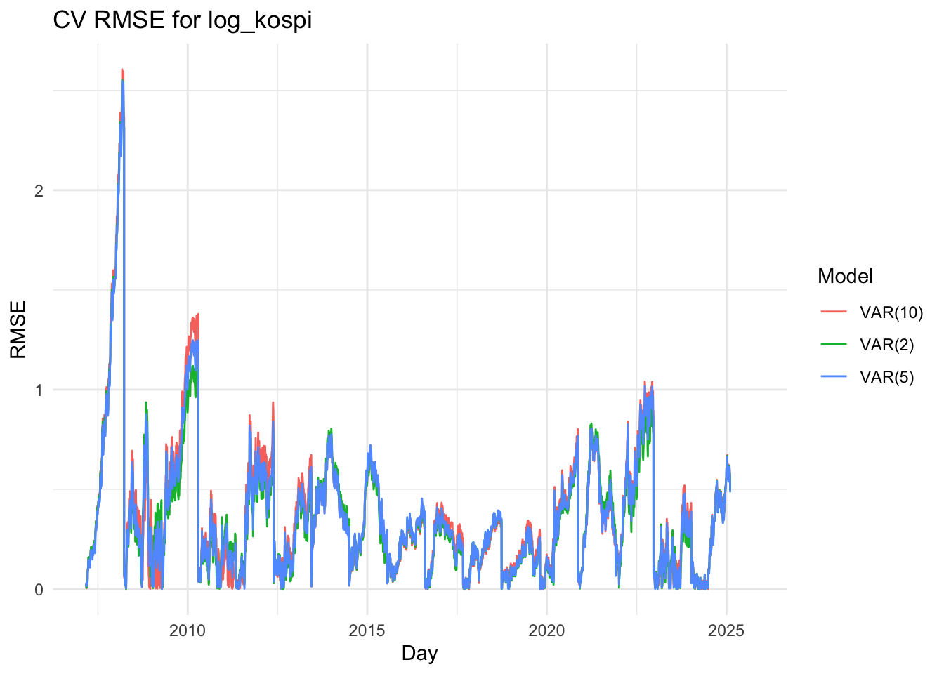
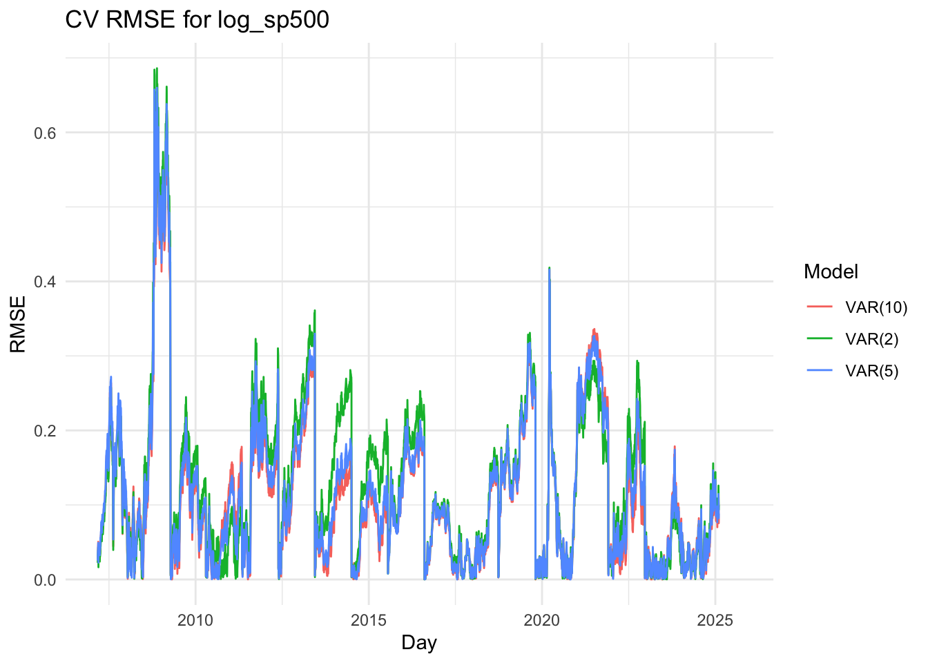
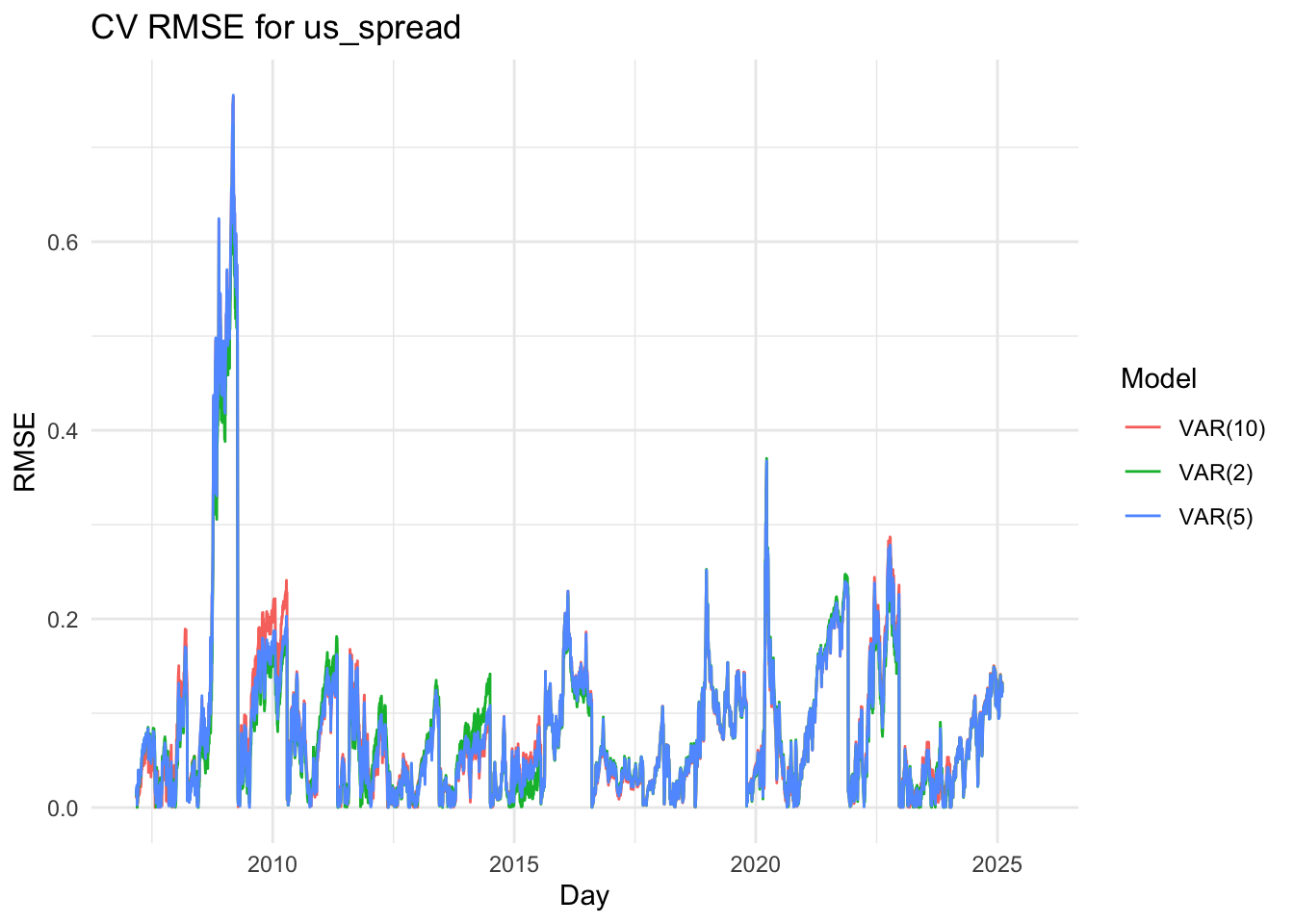
The VAR(2) model captures the short-term dynamics among the variables efficiently. The U.S. spread (us_spread) equation is mainly driven by its own lagged values, while both the Korean and U.S. stock indices (log_kospi and log_sp500) show strong dependence on their own past values and some cross-market effects. Most coefficients are statistically significant, and the model achieves a high R-squared (above 0.999) with low residual correlations, indicating a good fit and stable dynamics (all roots below one).

The VAR(5) model slightly improves the overall fit, as reflected by a marginal increase in log-likelihood and a small reduction in residual variance. Some additional lag terms, especially for the stock market variables, become significant, suggesting that the model captures medium-term interdependencies between the U.S. and Korean markets. However, several higher-order lag coefficients remain insignificant, implying that the added complexity provides limited explanatory gain.

The VAR(10) model, while achieving the highest log-likelihood, shows minimal improvement in explanatory power relative to the VAR(5) model. Many of the higher-order lag terms are statistically insignificant, and the R-squared values remain nearly identical to those of the simpler models. This indicates potential overfitting, as the model includes many parameters without substantial improvement in predictive accuracy.

Code

n=length(df1$log_sp500) 
k=1480 #1480
#n-k=4440; 4440/252=17.619
rmse1 <- matrix(NA, 4440,3) #here 4440 is n-k
rmse2 <- matrix(NA, 4440,3)
rmse3 <- matrix(NA,4440,3) #here n-k / 252 = 4440/252 =17.619
year<-c()
ts_obj <- ts(df1[, c(2,5,6)], start=decimal_date(as.Date("2000-12-18",format = "%Y-%m-%d")),frequency = 252)
st <- tsp(ts_obj)[1]+(k-1)/252 
for(i in 1:17) #here 17 is (n-k ) / 252 = 4440/252 =17.619
{
  
  xtrain <- window(ts_obj, end=st + i-1)
  xtest <- window(ts_obj, start=st + (i-1) + 1/252, end=st + i)
  
  # first model p = 2 
  fit <- vars::VAR(xtrain, p=2, type='both')
  fcast <- predict(fit, n.ahead = 252)
  
  fspread<-fcast$fcst$us_spread
  fkospi<-fcast$fcst$log_kospi
  fsp<-fcast$fcst$log_sp500
  
  ff1<-data.frame(fspread[,1],fkospi[,1],fsp[,1]) 
  year<-st + (i-1) + 1/252 
  
  
  ff1<-ts(ff1,start=c(year,1),frequency = 252)
  
  a = 252*i-251 
  b= 252*i 
 
  rmse1[c(a:b),]  <-sqrt((ff1-xtest)^2)
  
  #second model p = 5
  fit2 <- vars::VAR(xtrain, p=5, type='both')
  fcast2 <- predict(fit2, n.ahead = 252)
  
  fspread2<-fcast2$fcst$us_spread
  fkospi2<-fcast2$fcst$log_kospi
  fsp2<-fcast2$fcst$log_sp500
  ff2<-data.frame(fspread2[,1],fkospi2[,1],fsp2[,1])
  
  year<-st + (i-1) + 1/252
  
  ff2<-ts(ff2,start=c(year,1),frequency = 252)
  
  a = 252*i-251
  b= 252*i
  rmse2[c(a:b),]  <-sqrt((ff2-xtest)^2)
  
  #third model p = 10
  fit3 <- vars::VAR(xtrain, p=10, type='both')
  fcast3 <- predict(fit3, n.ahead = 252)
  
  fspread3<-fcast3$fcst$us_spread
  fkospi3<-fcast3$fcst$log_kospi
  fsp3<-fcast3$fcst$log_sp500
  ff3<-data.frame(fspread3[,1],fkospi3[,1],fsp3[,1])
  
  year<-st + (i-1) + 1/252
  
  ff3<-ts(ff3,start=c(year,1),frequency = 252)
  
  a = 252*i-251
  b= 252*i
  rmse3[c(a:b),]  <-sqrt((ff3-xtest)^2)
}

Code

day_index = 1:4440
dates1 = as.Date(df1$Date[(k+1):n])
rmse1 = data.frame(day_index,dates1,rmse1)
names(rmse1) =c("Day","Date","log_kospi","log_sp500","us_spread")
rmse2 = data.frame(day_index,dates1,rmse2)
names(rmse2) =c("Day","Date","log_kospi","log_sp500","us_spread")
rmse3 = data.frame(day_index,dates1,rmse3)
names(rmse3) =c("Day","Date","log_kospi","log_sp500","us_spread")
rmse1$Model <- "VAR(2)"
rmse2$Model <- "VAR(5)"
rmse3$Model <- "VAR(10)"
rmse_combined <- rbind(rmse1, rmse2, rmse3)
rmse1$Model <- "VAR(2)"
rmse2$Model <- "VAR(5)"
rmse3$Model <- "VAR(10)"
rmse_combined <- rbind(rmse1, rmse2, rmse3)

Code

ggplot(data = rmse_combined, aes(x = Date, y = log_kospi, color = Model)) + 
  geom_line() +
  labs(
    title = "CV RMSE for log_kospi",
    x = "Day",
    y = "RMSE",
    color = "Model"
  ) +
  theme_minimal()

Code

ggplot(data = rmse_combined, aes(x = Date, y = log_sp500, color = Model)) + 
  geom_line() +
  labs(
    title = "CV RMSE for log_sp500",
    x = "Day",
    y = "RMSE",
    color = "Model"
  ) +
  theme_minimal()

Code

ggplot(data = rmse_combined, aes(x = Date, y = us_spread, color = Model)) + 
  geom_line() +
  labs(
    title = "CV RMSE for us_spread",
    x = "Day",
    y = "RMSE",
    color = "Model"
  ) +
  theme_minimal()

Code

var5<- VAR(ts_obj,p = 5,type= "both")
acf(residuals(var5))

The three line plots above show the RMSE values for three variables, comparing the VAR(2),VAR(5) and var(10) models. Although it’s somewhat difficult to clearly distinguish which model performs better based solely on the plots, the VAR(2) model appears to have slightly lower RMSE values overall. Therefore, I decided to proceed with the VAR(5) model for further analysis.

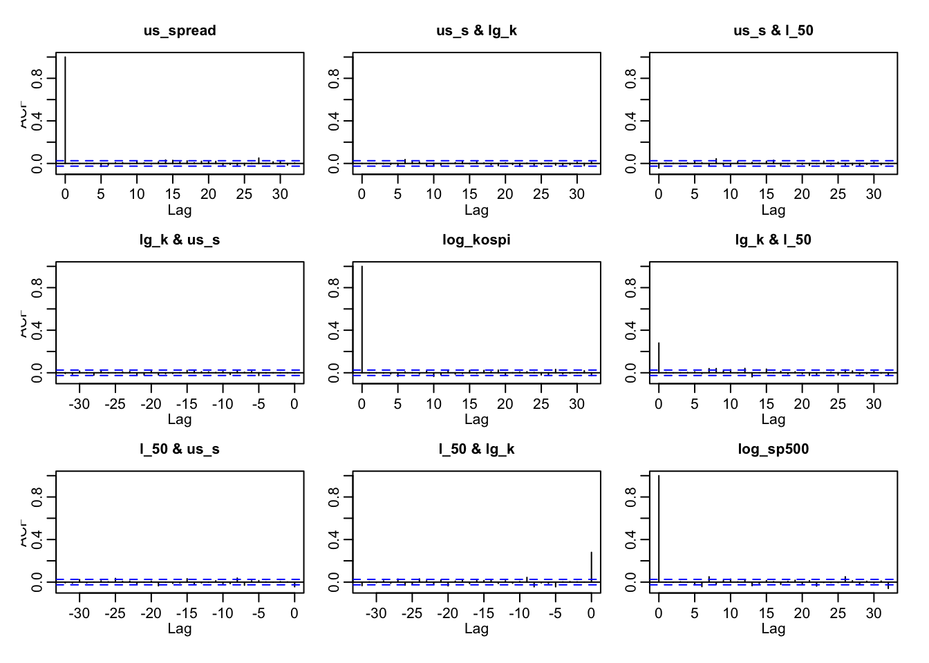
last plot is a acf plot for var(5) model’s residuals. From the plot, the residual autocorrelations are mostly within the 95% confidence bounds , except for a strong spike at lag 0, which simply reflects the correlation of each residual with itself. The absence of significant spikes beyond lag 0 suggests that the VAR(5) specification has successfully removed serial correlation from the system. This implies that the model order (p=5) is sufficient.

Overall, the ACF of the residuals confirms that the VAR(5) model is appropriately specified and that the residuals behave as approximately white noise.

Code

df1$Date <- as.Date(df1$Date)
n <- nrow(df1)

actual_frequency <- nrow(df1) / as.numeric(difftime(max(df1$Date), 
                                                     min(df1$Date), 
                                                     units = "days")) * 365.25

ts_obj <- ts(df1[, c("us_spread", "log_kospi", "log_sp500")],
             start = decimal_date(min(df1$Date)),
             frequency = round(actual_frequency))



h <- 504
fcast <- forecast(var5, h = h)


hist_dates <- df1$Date

last_date <- max(df1$Date)

all_future_dates <- seq(last_date + 1, by = "day", length.out = 1000)
future_weekdays <- all_future_dates[!weekdays(all_future_dates) %in% c("Saturday", "Sunday")]
fcast_dates <- head(future_weekdays, h)


fig1 <- plot_ly() %>%
  add_lines(
    x = tail(hist_dates, 2500),
    y = tail(df1$us_spread, 2500),
    name = "Historical",
    line = list(color = "black", width = 1),
    hovertemplate = "%{x|%Y-%m-%d}<br>%{y:.4f}<extra></extra>"
  ) %>%
  add_lines(
    x = fcast_dates,
    y = as.numeric(fcast$forecast$us_spread$mean),
    name = "Forecast",
    line = list(color = "blue", width = 2),
    hovertemplate = "%{x|%Y-%m-%d}<br>%{y:.4f}<extra></extra>"
  ) %>%
  add_ribbons(
    x = fcast_dates,
    ymin = as.numeric(fcast$forecast$us_spread$lower[,2]),
    ymax = as.numeric(fcast$forecast$us_spread$upper[,2]),
    name = "95% CI",
    line = list(color = "transparent"),
    hoverinfo = "skip"
  ) %>%
  add_ribbons(
    x = fcast_dates,
    ymin = as.numeric(fcast$forecast$us_spread$lower[,1]),
    ymax = as.numeric(fcast$forecast$us_spread$upper[,1]),
    name = "80% CI",
    line = list(color = "transparent"),
    hoverinfo = "skip"
  ) %>%
  layout(
    title = "VAR(5) Forecast for US Spread",
    xaxis = list(
      title = "Year",
      type = "date",
      tickformat = "%Y",     
      dtick = "M12"         
    ),
    yaxis = list(title = "US Spread"),
    hovermode = "x unified"
  )


fig2 <- plot_ly() %>%
  add_lines(
    x = tail(hist_dates, 2500),
    y = exp(tail(df1$log_kospi, 2500)),
    name = "Historical",
    line = list(color = "black", width = 1),
    hovertemplate = "%{x|%Y-%m-%d}<br>%{y:.2f}<extra></extra>"
  ) %>%
  add_lines(
    x = fcast_dates,
    y = exp(as.numeric(fcast$forecast$log_kospi$mean)),
    name = "Forecast",
    line = list(color = "blue", width = 2),
    hovertemplate = "%{x|%Y-%m-%d}<br>%{y:.2f}<extra></extra>"
  ) %>%
  add_ribbons(
    x = fcast_dates,
    ymin = exp(as.numeric(fcast$forecast$log_kospi$lower[,2])),
    ymax = exp(as.numeric(fcast$forecast$log_kospi$upper[,2])),
    name = "95% CI",
    line = list(color = "transparent"),
    hoverinfo = "skip"
  ) %>%
  add_ribbons(
    x = fcast_dates,
    ymin = exp(as.numeric(fcast$forecast$log_kospi$lower[,1])),
    ymax = exp(as.numeric(fcast$forecast$log_kospi$upper[,1])),
    name = "80% CI",
    line = list(color = "transparent"),
    hoverinfo = "skip"
  ) %>%
  layout(
    title = "VAR(5) Forecast for KOSPI",
    xaxis = list(
      title = "Year",
      type = "date",
      tickformat = "%Y",
      dtick = "M12"
    ),
    yaxis = list(title = "KOSPI Index"),
    hovermode = "x unified"
  )


fig3 <- plot_ly() %>%
  add_lines(
    x = tail(hist_dates, 2500),
    y = exp(tail(df1$log_sp500, 2500)),
    name = "Historical",
    line = list(color = "black", width = 1),
    hovertemplate = "%{x|%Y-%m-%d}<br>%{y:.2f}<extra></extra>"
  ) %>%
  add_lines(
    x = fcast_dates,
    y = exp(as.numeric(fcast$forecast$log_sp500$mean)),
    name = "Forecast",
    line = list(color = "blue", width = 2),
    hovertemplate = "%{x|%Y-%m-%d}<br>%{y:.2f}<extra></extra>"
  ) %>%
  add_ribbons(
    x = fcast_dates,
    ymin = exp(as.numeric(fcast$forecast$log_sp500$lower[,2])),
    ymax = exp(as.numeric(fcast$forecast$log_sp500$upper[,2])),
    name = "95% CI",
    line = list(color = "transparent"),
    hoverinfo = "skip"
  ) %>%
  add_ribbons(
    x = fcast_dates,
    ymin = exp(as.numeric(fcast$forecast$log_sp500$lower[,1])),
    ymax = exp(as.numeric(fcast$forecast$log_sp500$upper[,1])),
    name = "80% CI",
    line = list(color = "transparent"),
    hoverinfo = "skip"
  ) %>%
  layout(
    title = "VAR(5) Forecast for S&P 500",
    xaxis = list(
      title = "Year",
      type = "date",
      tickformat = "%Y",
      dtick = "M12"
    ),
    yaxis = list(title = "S&P 500 Index"),
    hovermode = "x unified"
  )

fig1

Code

fig2

Code

fig3

From the forecast plot, the VAR model demonstrates a good fit, accurately capturing the patterns of past data and projecting trends for the next two years. The model forecasts an increase in the U.S. 3-year and 10-year spreads as well as the S&P 500 index, while predicting an opposite movement for the KOSPI index.

This result is both interesting and economically reasonable. As the U.S. yield spreads rise, investors are likely to favor U.S. dollar–denominated assets, leading to a stronger dollar. However, this appreciation of the USD tends to weaken the Korean won (KRW), which in turn exerts downward pressure on the KOSPI index.

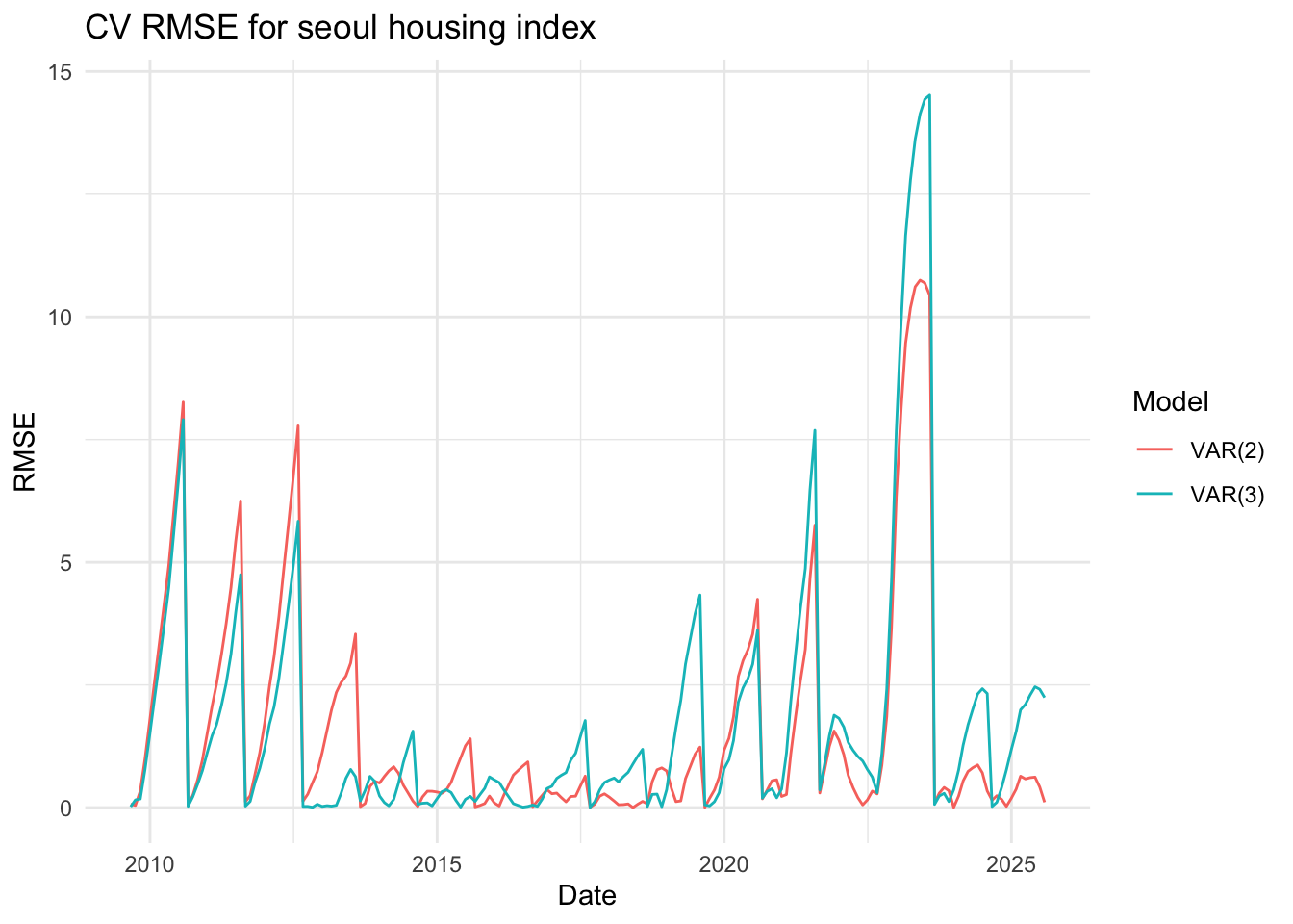
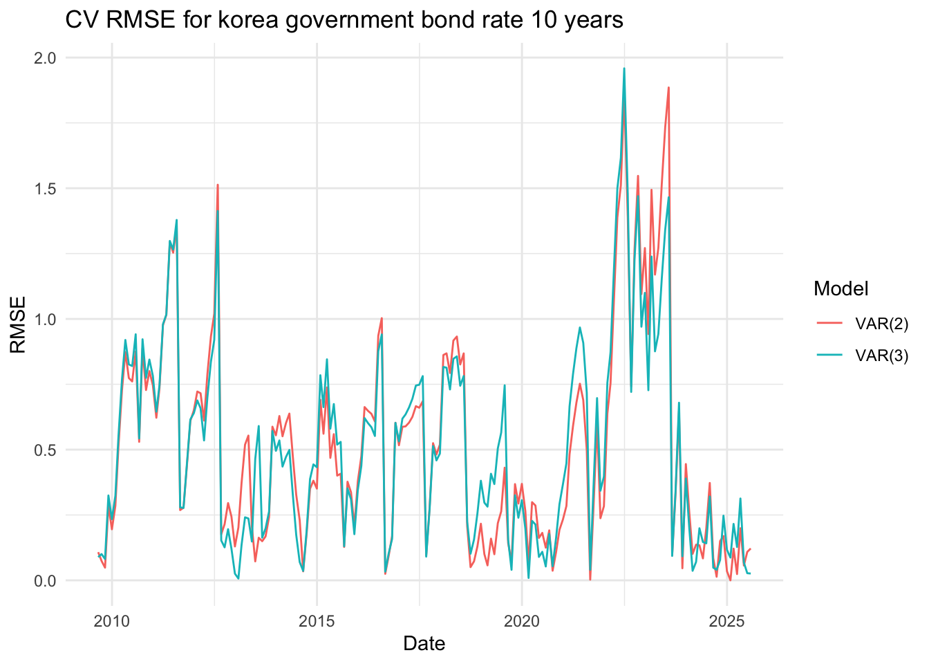
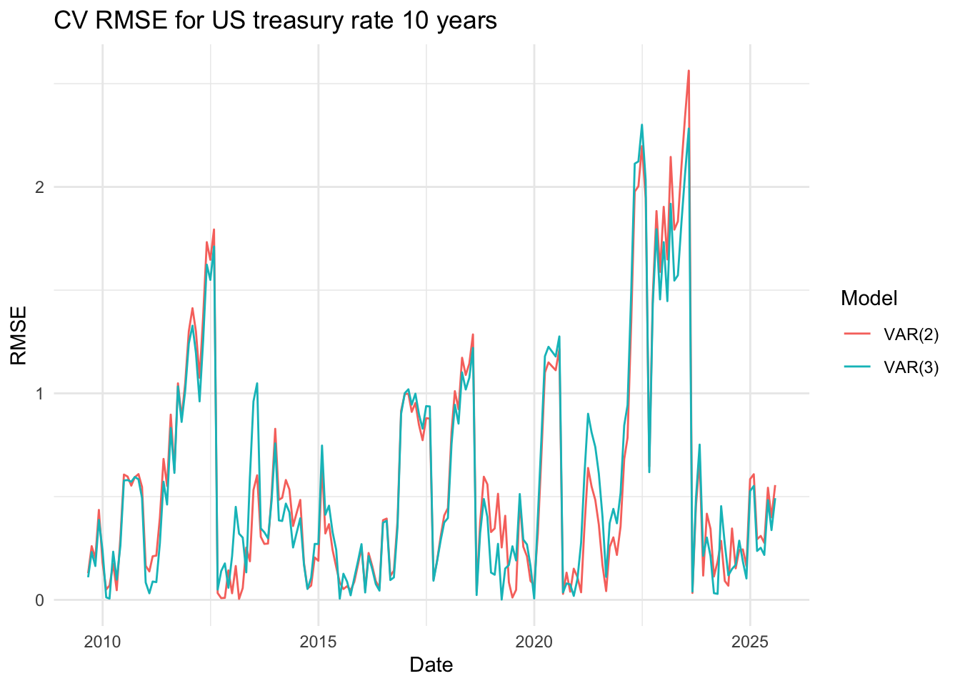
US treasury yield curve 10 Years, South Korea government bond rate 10Years, seoul housing index

data cleaning process

Code

kor_yield_10<- kor_yield%>%
  dplyr::select(Date,KR_10Y)
kor_yield_monthly <- kor_yield_10 %>%
  mutate(year_month = floor_date(Date, "month")) %>%
  group_by(year_month) %>%
  slice_tail(n = 1) %>%
  ungroup() %>%
  mutate(Date = ceiling_date(year_month, "month") - days(1))%>%
  dplyr::select(Date,KR_10Y)


us_yield_10<- us_yield%>%
  dplyr::select(Date,US_10Y)
us_yield_monthly <- us_yield_10 %>%
  mutate(year_month = floor_date(Date, "month")) %>%
  group_by(year_month) %>%
  slice_tail(n = 1) %>%
  ungroup() %>%
  mutate(Date = ceiling_date(year_month, "month") - days(1))%>%
  dplyr::select(Date,US_10Y)

df2<- housing%>%
  left_join(kor_yield_monthly,by = "Date")%>%
  left_join(us_yield_monthly, by = "Date")

start_year_df2  <- year(min(df2$Date))
start_month_df2 <- month(min(df2$Date))

Code

p2 <- plot_ly(df2, x = ~Date, y = ~housing, type = 'scatter', mode = 'lines',
              name = "Seoul housing Index") %>%
  layout(yaxis = list(title = "Seoul housing Index", titlefont = list(size = 14), tickfont = list(size = 12)))

p3 <- plot_ly(df2, x = ~Date, y = ~KR_10Y, type = 'scatter', mode = 'lines',
              name = "South Korea government bond yield rate(10years)") %>%
  layout(yaxis = list(title = "South Korea yield rate(10years)", titlefont = list(size = 14), tickfont = list(size = 12)))

p4 <- plot_ly(df2, x = ~Date, y = ~US_10Y, type = 'scatter', mode = 'lines',
              name = "U.S. treasury bond yield rate(10years)") %>%
  layout(yaxis = list(title = "KRW/USD spot rate", titlefont = list(size = 14)))

subplot( p2, p3,p4, nrows = 3, shareX = TRUE, titleX = TRUE) %>%
  layout(title = list(text = "U.S. treasury bond yield rate(10years)"))

Code

new_df2<- df2[,c(2:4)]
df2.ts<-ts(new_df2,star=decimal_date(as.Date("2003-11-30",format = "%Y-%m-%d")),frequency = 12)
VARselect(df2.ts, lag.max=10, type="both")

$selection
AIC(n)  HQ(n)  SC(n) FPE(n) 
     3      3      2      3 

$criteria
                   1             2             3             4             5
AIC(n) -7.2354237514 -8.6966493085 -8.7538981175 -8.6951961691 -8.6376638957
HQ(n)  -7.1506390633 -8.5609938075 -8.5673718036 -8.4577990423 -8.3493959561
SC(n)  -7.0247393128 -8.3595542068 -8.2903923526 -8.1052797410 -7.9213368045
FPE(n)  0.0007206133  0.0001671558  0.0001578714  0.0001674462  0.0001774111
                   6             7             8             9            10
AIC(n) -8.5859212103 -8.5718104042 -8.5100114868 -8.4743238217 -8.4526816818
HQ(n)  -8.2467824578 -8.1818008388 -8.0691311085 -7.9825726306 -7.9100596778
SC(n)  -7.7431834559 -7.6026619867 -7.4144524061 -7.2523540779 -7.1043012748
FPE(n)  0.0001869059  0.0001896626  0.0002018927  0.0002094105  0.0002142223

From parameter selction process, two parameters were suggested; p = 2,3

Code

summary(fit <- VAR(new_df2, p=2, type="both"))


VAR Estimation Results:
========================= 
Endogenous variables: housing, KR_10Y, US_10Y 
Deterministic variables: both 
Sample size: 259 
Log Likelihood: 45.633 
Roots of the characteristic polynomial:
0.965 0.947 0.9063 0.9063 0.1358 0.02788
Call:
VAR(y = new_df2, p = 2, type = "both")


Estimation results for equation housing: 
======================================== 
housing = housing.l1 + KR_10Y.l1 + US_10Y.l1 + housing.l2 + KR_10Y.l2 + US_10Y.l2 + const + trend 

            Estimate Std. Error t value Pr(>|t|)    
housing.l1  1.858502   0.030694  60.549  < 2e-16 ***
KR_10Y.l1   0.151384   0.088160   1.717 0.087186 .  
US_10Y.l1  -0.088694   0.081804  -1.084 0.279307    
housing.l2 -0.870774   0.031228 -27.884  < 2e-16 ***
KR_10Y.l2  -0.112900   0.087955  -1.284 0.200459    
US_10Y.l2   0.043591   0.080985   0.538 0.590873    
const       0.789500   0.236201   3.342 0.000957 ***
trend       0.002052   0.001134   1.810 0.071557 .  
---
Signif. codes:  0 '***' 0.001 '**' 0.01 '*' 0.05 '.' 0.1 ' ' 1


Residual standard error: 0.269 on 251 degrees of freedom
Multiple R-Squared: 0.9996, Adjusted R-squared: 0.9996 
F-statistic: 9.185e+04 on 7 and 251 DF,  p-value: < 2.2e-16 


Estimation results for equation KR_10Y: 
======================================= 
KR_10Y = housing.l1 + KR_10Y.l1 + US_10Y.l1 + housing.l2 + KR_10Y.l2 + US_10Y.l2 + const + trend 

             Estimate Std. Error t value Pr(>|t|)    
housing.l1  0.0546272  0.0257766   2.119 0.035051 *  
KR_10Y.l1   0.7155168  0.0740362   9.664  < 2e-16 ***
US_10Y.l1   0.2772800  0.0686984   4.036 7.22e-05 ***
housing.l2 -0.0489818  0.0262253  -1.868 0.062965 .  
KR_10Y.l2   0.2164915  0.0738636   2.931 0.003691 ** 
US_10Y.l2  -0.2467968  0.0680101  -3.629 0.000345 ***
const      -0.1526568  0.1983593  -0.770 0.442262    
trend      -0.0014886  0.0009524  -1.563 0.119324    
---
Signif. codes:  0 '***' 0.001 '**' 0.01 '*' 0.05 '.' 0.1 ' ' 1


Residual standard error: 0.2259 on 251 degrees of freedom
Multiple R-Squared: 0.9717, Adjusted R-squared: 0.9709 
F-statistic:  1233 on 7 and 251 DF,  p-value: < 2.2e-16 


Estimation results for equation US_10Y: 
======================================= 
US_10Y = housing.l1 + KR_10Y.l1 + US_10Y.l1 + housing.l2 + KR_10Y.l2 + US_10Y.l2 + const + trend 

             Estimate Std. Error t value Pr(>|t|)    
housing.l1  0.0373124  0.0282106   1.323   0.1872    
KR_10Y.l1  -0.0004244  0.0810271  -0.005   0.9958    
US_10Y.l1   1.0356735  0.0751852  13.775   <2e-16 ***
housing.l2 -0.0468702  0.0287016  -1.633   0.1037    
KR_10Y.l2   0.1057487  0.0808381   1.308   0.1920    
US_10Y.l2  -0.1373780  0.0744319  -1.846   0.0661 .  
const       0.3944815  0.2170893   1.817   0.0704 .  
trend       0.0025613  0.0010423   2.457   0.0147 *  
---
Signif. codes:  0 '***' 0.001 '**' 0.01 '*' 0.05 '.' 0.1 ' ' 1


Residual standard error: 0.2473 on 251 degrees of freedom
Multiple R-Squared: 0.9549, Adjusted R-squared: 0.9536 
F-statistic: 758.9 on 7 and 251 DF,  p-value: < 2.2e-16 



Covariance matrix of residuals:
           housing   KR_10Y     US_10Y
housing  0.0723737 0.007764 -0.0005108
KR_10Y   0.0077642 0.051041  0.0303960
US_10Y  -0.0005108 0.030396  0.0611356

Correlation matrix of residuals:
          housing KR_10Y    US_10Y
housing  1.000000 0.1277 -0.007679
KR_10Y   0.127745 1.0000  0.544137
US_10Y  -0.007679 0.5441  1.000000

Code

summary(fit <- VAR(new_df2, p=3, type="both"))


VAR Estimation Results:
========================= 
Endogenous variables: housing, KR_10Y, US_10Y 
Deterministic variables: both 
Sample size: 258 
Log Likelihood: 61.065 
Roots of the characteristic polynomial:
0.9749 0.9524 0.8751 0.8751 0.3857 0.3857 0.3273 0.3273 0.2444
Call:
VAR(y = new_df2, p = 3, type = "both")


Estimation results for equation housing: 
======================================== 
housing = housing.l1 + KR_10Y.l1 + US_10Y.l1 + housing.l2 + KR_10Y.l2 + US_10Y.l2 + housing.l3 + KR_10Y.l3 + US_10Y.l3 + const + trend 

            Estimate Std. Error t value Pr(>|t|)    
housing.l1  2.043800   0.061604  33.176   <2e-16 ***
KR_10Y.l1   0.129385   0.087402   1.480   0.1401    
US_10Y.l1  -0.056602   0.079288  -0.714   0.4760    
housing.l2 -1.247417   0.117832 -10.586   <2e-16 ***
KR_10Y.l2  -0.250874   0.105057  -2.388   0.0177 *  
US_10Y.l2  -0.100860   0.106653  -0.946   0.3452    
housing.l3  0.194519   0.061320   3.172   0.0017 ** 
KR_10Y.l3   0.148010   0.086738   1.706   0.0892 .  
US_10Y.l3   0.131469   0.080463   1.634   0.1036    
const       0.574709   0.236642   2.429   0.0159 *  
trend       0.001537   0.001143   1.345   0.1799    
---
Signif. codes:  0 '***' 0.001 '**' 0.01 '*' 0.05 '.' 0.1 ' ' 1


Residual standard error: 0.2592 on 247 degrees of freedom
Multiple R-Squared: 0.9996, Adjusted R-squared: 0.9996 
F-statistic: 6.814e+04 on 10 and 247 DF,  p-value: < 2.2e-16 


Estimation results for equation KR_10Y: 
======================================= 
KR_10Y = housing.l1 + KR_10Y.l1 + US_10Y.l1 + housing.l2 + KR_10Y.l2 + US_10Y.l2 + housing.l3 + KR_10Y.l3 + US_10Y.l3 + const + trend 

             Estimate Std. Error t value Pr(>|t|)    
housing.l1  0.1737428  0.0533434   3.257  0.00128 ** 
KR_10Y.l1   0.6915471  0.0756818   9.138  < 2e-16 ***
US_10Y.l1   0.2973998  0.0686561   4.332 2.15e-05 ***
housing.l2 -0.2956775  0.1020320  -2.898  0.00409 ** 
KR_10Y.l2   0.1876121  0.0909700   2.062  0.04022 *  
US_10Y.l2  -0.2534877  0.0923513  -2.745  0.00650 ** 
housing.l3  0.1301736  0.0530975   2.452  0.01492 *  
KR_10Y.l3   0.0376365  0.0751073   0.501  0.61674    
US_10Y.l3  -0.0001830  0.0696738  -0.003  0.99791    
const      -0.2884201  0.2049101  -1.408  0.16052    
trend      -0.0020085  0.0009898  -2.029  0.04350 *  
---
Signif. codes:  0 '***' 0.001 '**' 0.01 '*' 0.05 '.' 0.1 ' ' 1


Residual standard error: 0.2244 on 247 degrees of freedom
Multiple R-Squared: 0.9723, Adjusted R-squared: 0.9712 
F-statistic: 867.2 on 10 and 247 DF,  p-value: < 2.2e-16 


Estimation results for equation US_10Y: 
======================================= 
US_10Y = housing.l1 + KR_10Y.l1 + US_10Y.l1 + housing.l2 + KR_10Y.l2 + US_10Y.l2 + housing.l3 + KR_10Y.l3 + US_10Y.l3 + const + trend 

            Estimate Std. Error t value Pr(>|t|)    
housing.l1  0.131134   0.058612   2.237   0.0262 *  
KR_10Y.l1   0.004759   0.083156   0.057   0.9544    
US_10Y.l1   1.049307   0.075436  13.910   <2e-16 ***
housing.l2 -0.250432   0.112109  -2.234   0.0264 *  
KR_10Y.l2   0.141081   0.099954   1.411   0.1594    
US_10Y.l2  -0.223614   0.101472  -2.204   0.0285 *  
housing.l3  0.112508   0.058341   1.928   0.0549 .  
KR_10Y.l3  -0.063515   0.082525  -0.770   0.4422    
US_10Y.l3   0.093791   0.076555   1.225   0.2217    
const       0.265366   0.225147   1.179   0.2397    
trend       0.001936   0.001088   1.780   0.0762 .  
---
Signif. codes:  0 '***' 0.001 '**' 0.01 '*' 0.05 '.' 0.1 ' ' 1


Residual standard error: 0.2466 on 247 degrees of freedom
Multiple R-Squared: 0.9557, Adjusted R-squared: 0.9539 
F-statistic: 532.4 on 10 and 247 DF,  p-value: < 2.2e-16 



Covariance matrix of residuals:
          housing   KR_10Y    US_10Y
housing  0.067164 0.005595 -0.002621
KR_10Y   0.005595 0.050359  0.029895
US_10Y  -0.002621 0.029895  0.060797

Correlation matrix of residuals:
         housing KR_10Y   US_10Y
housing  1.00000 0.0962 -0.04102
KR_10Y   0.09620 1.0000  0.54028
US_10Y  -0.04102 0.5403  1.00000

In the VAR(2) model, the housing variable is primarily driven by its own past values, with highly significant coefficients for its first and second lags (positive and negative, respectively), implying mean-reverting dynamics. Korean and U.S. long-term interest rates (KR_10Y and US_10Y) have only weak short-run effects on housing, as most of their coefficients are statistically insignificant. The KR_10Y equation shows strong persistence—its own first and second lags are significant and positive—and a significant influence from the U.S. 10-year yield, suggesting cross-country linkages in bond markets. The U.S. yield (US_10Y) equation confirms high persistence as well, with its first lag strongly significant, while the trend term is also positive and significant, indicating a gradual upward drift. Residual correlations show moderate co-movement between KR_10Y and US_10Y (ρ ≈ 0.54) but only weak links between interest rates and housing.

The VAR(3) model slightly improves the log-likelihood (from 45.63 to 61.07) and marginally lowers residual variances, suggesting a better fit. Additional lag terms introduce some new dynamics: the third lag of housing becomes positive and significant, implying cyclical adjustment, while the second lag of KR_10Y is now significant and negative, and the third lag positive, showing alternating effects on housing. In the KR_10Y equation, housing’s first, second, and third lags all become significant, reinforcing feedback from the housing market to Korean yields. The U.S. yield equation remains dominated by its own autoregressive terms, with limited cross-effects, though housing’s influence is now slightly stronger. Overall, the VAR(3) captures more complex intertemporal relationships and richer lag structures, but the incremental explanatory gain over VAR(2) is small, and most new coefficients are marginally significant.

Code

df2$Date <- as.Date(df2$Date)

series_names <- c("housing", "KR_10Y", "US_10Y")



ts_obj <- ts(df2[, series_names],
             start = c(year(df2$Date[1]), month(df2$Date[1])),
             frequency = 12)


n <- nrow(df2)
k<- 69
h <- 12
n_k <- n - k
num_blocks <- floor(n_k / h)

rmse2 <- matrix(NA_real_, n_k, 3)   
rmse3 <- matrix(NA_real_, n_k, 3)  


st <- tsp(ts_obj)[1] + (k - 1) / 12


for (i in 1:num_blocks) {
  xtrain <- window(ts_obj, end = st + i - 1)

  xtest  <- window(ts_obj,
                   start = st + (i - 1) + 1/12,
                   end   = st + i)

  if (NROW(xtest) != h) next  

  fit2   <- vars::VAR(xtrain, p = 2, type = "both")
  fcast2 <- predict(fit2, n.ahead = h)

  ff2 <- cbind(
    fcast2$fcst$housing[, 1],
    fcast2$fcst$KR_10Y [, 1],
    fcast2$fcst$US_10Y [, 1]
  )

  year <- st + (i - 1) + 1/12
  ff2  <- ts(ff2, start = c(year, 1), frequency = 12)

  a <- 12 * i - 11
  b <- 12 * i
  rmse2[a:b, ] <- sqrt((ff2 - xtest)^2)

  fit3   <- vars::VAR(xtrain, p = 3, type = "both")
  fcast3 <- predict(fit3, n.ahead = h)

  ff3 <- cbind(
    fcast3$fcst$housing[, 1],
    fcast3$fcst$KR_10Y [, 1],
    fcast3$fcst$US_10Y [, 1]
  )

  ff3 <- ts(ff3, start = c(year, 1), frequency = 12)

  rmse3[a:b, ] <- sqrt((ff3 - xtest)^2)
}

colnames(rmse2) <- series_names
colnames(rmse3) <- series_names

month_index <- 1:n_k
dates1 <- as.Date(df2$Date[(k + 1):n])

if (length(dates1) < n_k) {
  dates1 <- c(dates1, rep(as.Date(NA), n_k - length(dates1)))
} else if (length(dates1) > n_k) {
  dates1 <- dates1[1:n_k]
}

rmse2_df <- data.frame(month_index, dates1, rmse2, row.names = NULL)
names(rmse2_df) <- c("Month","Date", series_names)
rmse2_df$Model <- "VAR(2)"

rmse3_df <- data.frame(month_index, dates1, rmse3, row.names = NULL)
names(rmse3_df) <- c("Month","Date", series_names)
rmse3_df$Model <- "VAR(3)"

rmse_combined <- rbind(rmse2_df, rmse3_df)

Code

ggplot(data = rmse_combined, aes(x = Date, y = housing, color = Model)) +
  geom_line() +
  labs(
    title = "CV RMSE for seoul housing index",
    x = "Date",
    y = "RMSE",
    color = "Model"
  ) +
  theme_minimal()

Code

ggplot(data = rmse_combined, aes(x = Date, y = KR_10Y, color = Model)) +
  geom_line() +
  labs(
    title = "CV RMSE for korea government bond rate 10 years",
    x = "Date",
    y = "RMSE",
    color = "Model"
  ) +
  theme_minimal()

Code

ggplot(data = rmse_combined, aes(x = Date, y = US_10Y, color = Model)) +
  geom_line() +
  labs(
    title = "CV RMSE for US treasury rate 10 years",
    x = "Date",
    y = "RMSE",
    color = "Model"
  ) +
  theme_minimal()

Code

var1<- VAR(ts_obj,p = 2,type= "both")
acf(residuals(var1))

The three line plots above show the RMSE values for three variables, comparing the VAR(2) and VAR(3) models. Although it’s somewhat difficult to clearly distinguish which model performs better based solely on the plots, the VAR(2) model appears to have slightly lower RMSE values overall. Therefore, I decided to proceed with the VAR(2) model for further analysis.

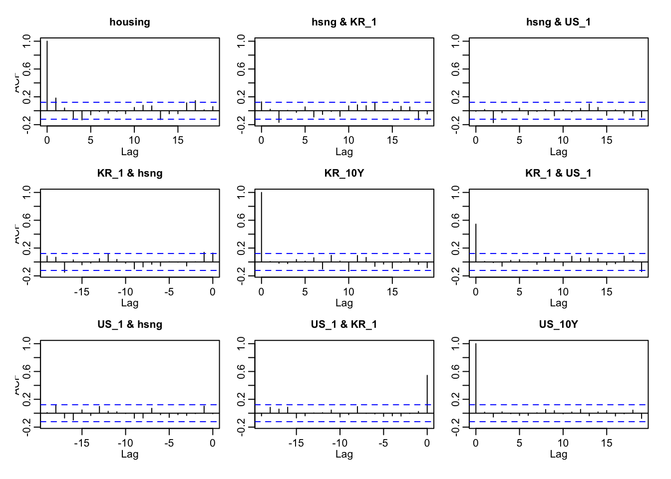
last plot is a acf plot for var(2) model’s residuals. From the plot, the residual autocorrelations are mostly within the 95% confidence bounds , except for a strong spike at lag 0, which simply reflects the correlation of each residual with itself. The absence of significant spikes beyond lag 0 suggests that the VAR(2) specification has successfully removed serial correlation from the system. This implies that the model order (p=2) is sufficient.

Overall, the ACF of the residuals confirms that the VAR(2) model is appropriately specified and that the residuals behave as approximately white noise.

Code

h <- 36
fcast <- forecast(var1, h = h)

hist_dates <- df2$Date


last_date <- max(df2$Date)
fcast_dates <- seq(last_date, by = "month", length.out = h + 1)[-1]
fcast_dates <- ceiling_date(fcast_dates, "month") - days(1)

fig1 <- plot_ly() %>%

  add_lines(
    x = tail(hist_dates, 100),
    y = tail(df2$housing, 100),
    name = "Historical",
    line = list(color = "black", width = 1),
    hovertemplate = "%{x|%Y-%m}<br>%{y:.2f}<extra></extra>"
  ) %>%

  add_lines(
    x = fcast_dates,
    y = as.numeric(fcast$forecast$housing$mean),
    name = "Forecast",
    line = list(color = "blue", width = 2),
    hovertemplate = "%{x|%Y-%m}<br>%{y:.2f}<extra></extra>"
  ) %>%

  add_ribbons(
    x = fcast_dates,
    ymin = as.numeric(fcast$forecast$housing$lower[,2]),
    ymax = as.numeric(fcast$forecast$housing$upper[,2]),
    name = "95% CI",
    line = list(color = "transparent"),
    hoverinfo = "skip"
  ) %>%
  # 80% CI
  add_ribbons(
    x = fcast_dates,
    ymin = as.numeric(fcast$forecast$housing$lower[,1]),
    ymax = as.numeric(fcast$forecast$housing$upper[,1]),
    name = "80% CI",
    line = list(color = "transparent"),
    hoverinfo = "skip"
  ) %>%
  layout(
    title = "VAR(2) Forecast for Housing",
    xaxis = list(
      title = "Year",
      type = "date",
      tickformat = "%Y",
      dtick = "M12"
    ),
    yaxis = list(title = "Housing Index"),
    hovermode = "x unified"
  )

fig2 <- plot_ly() %>%
  add_lines(
    x = tail(hist_dates, 100),
    y = tail(df2$KR_10Y, 100),
    name = "Historical",
    line = list(color = "black", width = 1),
    hovertemplate = "%{x|%Y-%m}<br>%{y:.2f}%<extra></extra>"
  ) %>%
  add_lines(
    x = fcast_dates,
    y = as.numeric(fcast$forecast$KR_10Y$mean),
    name = "Forecast",
    line = list(color = "blue", width = 2),
    hovertemplate = "%{x|%Y-%m}<br>%{y:.2f}%<extra></extra>"
  ) %>%
  add_ribbons(
    x = fcast_dates,
    ymin = as.numeric(fcast$forecast$KR_10Y$lower[,2]),
    ymax = as.numeric(fcast$forecast$KR_10Y$upper[,2]),
    name = "95% CI",
    line = list(color = "transparent"),
    hoverinfo = "skip"
  ) %>%
  add_ribbons(
    x = fcast_dates,
    ymin = as.numeric(fcast$forecast$KR_10Y$lower[,1]),
    ymax = as.numeric(fcast$forecast$KR_10Y$upper[,1]),
    name = "80% CI",
    line = list(color = "transparent"),
    hoverinfo = "skip"
  ) %>%
  layout(
    title = "VAR(2) Forecast for Korea 10Y Yield",
    xaxis = list(
      title = "Year",
      type = "date",
      tickformat = "%Y",
      dtick = "M12"
    ),
    yaxis = list(title = "Yield (%)"),
    hovermode = "x unified"
  )


fig3 <- plot_ly() %>%
  add_lines(
    x = tail(hist_dates, 100),
    y = tail(df2$US_10Y, 100),
    name = "Historical",
    line = list(color = "black", width = 1),
    hovertemplate = "%{x|%Y-%m}<br>%{y:.2f}%<extra></extra>"
  ) %>%
  add_lines(
    x = fcast_dates,
    y = as.numeric(fcast$forecast$US_10Y$mean),
    name = "Forecast",
    line = list(color = "blue", width = 2),
    hovertemplate = "%{x|%Y-%m}<br>%{y:.2f}%<extra></extra>"
  ) %>%
  add_ribbons(
    x = fcast_dates,
    ymin = as.numeric(fcast$forecast$US_10Y$lower[,2]),
    ymax = as.numeric(fcast$forecast$US_10Y$upper[,2]),
    name = "95% CI",
    line = list(color = "transparent"),
    hoverinfo = "skip"
  ) %>%
  add_ribbons(
    x = fcast_dates,
    ymin = as.numeric(fcast$forecast$US_10Y$lower[,1]),
    ymax = as.numeric(fcast$forecast$US_10Y$upper[,1]),
    name = "80% CI",
    line = list(color = "transparent"),
    hoverinfo = "skip"
  ) %>%
  layout(
    title = "VAR(2) Forecast for US 10Y Yield",
    xaxis = list(
      title = "Year",
      type = "date",
      tickformat = "%Y",
      dtick = "M12"
    ),
    yaxis = list(title = "Yield (%)"),
    hovermode = "x unified"
  )


fig1

Code

fig2

Code

fig3

The forecast suggests that yield curve rates are expected to decrease gradually over time, signaling a potential easing of monetary conditions. In contrast, the Seoul Residential Property Price Index is projected to increase, moving in the opposite direction. A decline in long-term yields often signals market expectations for lower policy rates in the future. Such expectations tend to stimulate the housing market, as lower interest rates reduce borrowing costs, making it cheaper to finance real estate purchases. Consequently, easier monetary conditions can lead to stronger demand and higher residential property prices.

SARIMAX model: USD/KRW spot rate ~ us-korea spread rate 3years+ us-korea spread rate 10years+ S&P500+ dollar index

data cleaning

Code

spread_3y_monthly <- us_kr_spreads_3y%>%
  mutate(year_month = floor_date(Date, "month")) %>%
  group_by(year_month) %>%
  slice_tail(n = 1) %>%
  ungroup() %>%
  mutate(Date = ceiling_date(year_month, "month") - days(1))%>%
    dplyr::select(Date,US_KR_3Y)


spread_10y_monthly <- us_kr_spreads_10y%>%
  mutate(year_month = floor_date(Date, "month")) %>%
  group_by(year_month) %>%
  slice_tail(n = 1) %>%
  ungroup() %>%
  mutate(Date = ceiling_date(year_month, "month") - days(1))%>%
  dplyr::select(Date,US_KR_10Y)


sp500_monthly <-
  sp500 %>%
  mutate(year_month = floor_date(Date, "month")) %>%
  group_by(year_month) %>%
  slice_tail(n = 1) %>%               
  ungroup() %>%
  mutate(Date = ceiling_date(year_month, "month") - days(1)) %>%  
  dplyr::select(Date, Close) %>%
  rename(sp500_close = Close) %>%
  arrange(Date) %>%
  mutate(
    return = sp500_close / lag(sp500_close) - 1,      
    log_return = log(sp500_close) - log(lag(sp500_close))
  )%>%
  dplyr::select(Date,sp500_close)


usd_monthly<-usd%>%
  mutate(year_month = floor_date(Date, "month")) %>%
  group_by(year_month) %>%
  slice_tail(n = 1) %>%
  ungroup() %>%
  mutate(Date = ceiling_date(year_month, "month") - days(1))%>%
  dplyr::select(Date,usd_index)

kor_monthly <- kr %>%
  mutate(year_month = floor_date(Date, "month")) %>%
  group_by(year_month) %>%
  slice_tail(n = 1) %>%
  ungroup() %>%
  mutate(Date = ceiling_date(year_month, "month") - days(1))%>%
  dplyr::select(Date,krw)





df3<- spread_3y_monthly%>%
  left_join(spread_10y_monthly,by = "Date")%>%
  left_join(sp500_monthly, by = "Date")%>%
  left_join(usd_monthly,by = "Date")%>%
  left_join(kor_monthly)

start_year_df3  <- year(min(df3$Date))
start_month_df3 <- month(min(df3$Date))

ts_krw <- ts(df3$krw, 
              star=decimal_date(as.Date("2000-12-01",format = "%Y-%m-%d")),frequency = 12)  

ts_log_krw <- ts(log(df3$krw), 
                  star=decimal_date(as.Date("2000-12-01",format = "%Y-%m-%d")),frequency = 12)

manual search utility function

Code

SARIMA.c <- function(p_range, d_range, q_range, P_range, D_range, Q_range, data) {
  
  # Set seasonal period
  s <- 12
  
  # Initialize results storage
  results_list <- list()
  
  # Iterate over parameter combinations
  for (p in p_range) {
    for (d in d_range) {
      for (q in q_range) {
        for (P in P_range) {
          for (D in D_range) {
            for (Q in Q_range) {
              
              # Apply parameter constraint to avoid overfitting
              if (p + d + q + P + D + Q <= 10) {
                tryCatch({
                  # Fit SARIMA model
                  model <- Arima(data, order = c(p, d, q), seasonal = c(P, D, Q))
                  
                  # Store results
                  results_list[[length(results_list) + 1]] <- c(p, d, q, P, D, Q, model$aic, model$bic, model$aicc)
                }, error = function(e) {
                  # Handle errors without breaking the loop
                  cat("Model failed for (p=", p, ", d=", d, ", q=", q, ", P=", P, ", D=", D, ", Q=", Q, ")\n")
                })
              }
            }
          }
        }
      }
    }
  }
  
  # Convert results to a tidy data frame
  results_df <- as.data.frame(do.call(rbind, results_list))
  colnames(results_df) <- c("p", "d", "q", "P", "D", "Q", "AIC", "BIC", "AICc")
  
  return(results_df)
}

Code

# arima 
ARIMA.c <- function(p_range, d_range, q_range, data,
                    include_drift = TRUE,
                    quiet = TRUE) {

  results <- list()

  for (p in p_range) {
    for (d in d_range) {
      for (q in q_range) {

        fit <- tryCatch(
          {
            forecast::Arima(
              y = data,
              order = c(p, d, q),
              include.drift = include_drift
            )
          },
          error = function(e) {
            if (!quiet) message(sprintf("Model failed for p=%d d=%d q=%d: %s", p, d, q, e$message))
            NULL
          }
        )

        if (!is.null(fit)) {
          results[[length(results) + 1L]] <- data.frame(
            p = p, d = d, q = q,
            AIC  = fit$aic,
            BIC  = fit$bic,
            AICc = fit$aicc,
            stringsAsFactors = FALSE
          )
        }
      }
    }
  }

  if (length(results) == 0L) {
    return(data.frame(
      p = integer(), d = integer(), q = integer(),
      AIC = double(), BIC = double(), AICc = double()
    ))
  }

  out <- do.call(rbind, results)
  rownames(out) <- NULL
  out[order(out$AIC), ]
}

log transformation

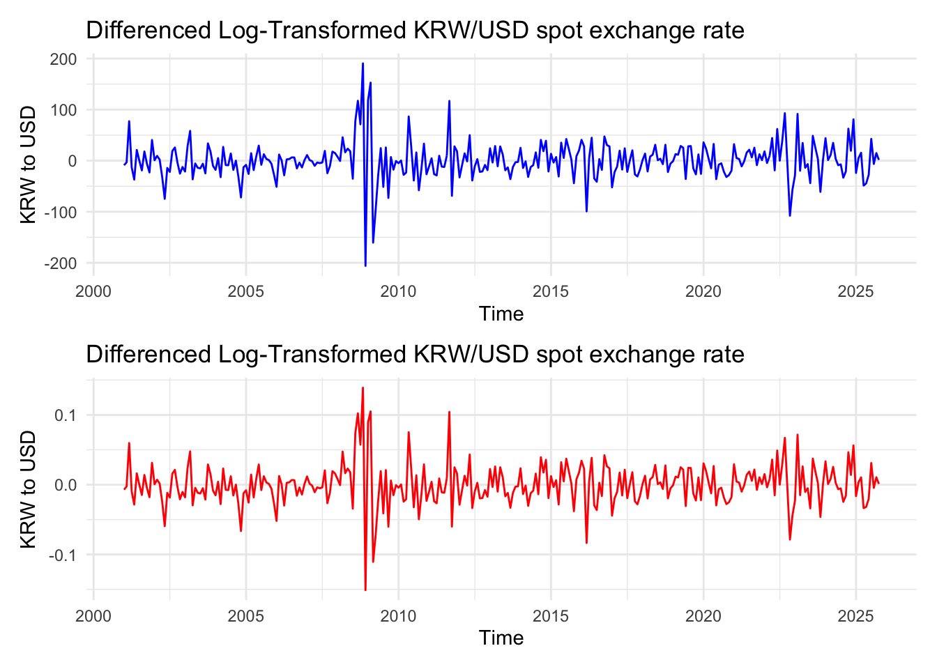
In EDA and univariate section, taking log for S&P500 index and USD index was better, so it will continue to use log transformation. however, here, FX rate needs to be checked

Code

diff_krw <- diff(ts_krw)
diff_log_krw <- diff(ts_log_krw)


p1 <- ggplot() +
  geom_line(aes(x = time(diff_krw), y = diff_krw), color = "blue") +
  labs(title = "Differenced Log-Transformed KRW/USD spot exchange rate",
       x = "Time",
       y = "KRW to USD") +
  theme_minimal()

p2 <- ggplot() +
  geom_line(aes(x = time(diff_log_krw), y = diff_log_krw), color = "red") +
  labs(title = "Differenced Log-Transformed KRW/USD spot exchange rate",
       x = "Time",
       y = "KRW to USD") +
  theme_minimal()




p1 / p2

from the plot, log transformation don’t give dramatical change, so for this model, original value for KRW/USD spot exchange rate will be used.

Code

p5 <- plot_ly(df3, x = ~Date, y = ~US_KR_3Y, type = "scatter", mode = "lines",
              name = "kor-us 3y bond spread rate") %>%
layout(yaxis = list(title = "kor-us 3y bond spread rate", titlefont = list(size = 14), tickfont = list(size = 12)))

p6 <- plot_ly(df3, x = ~Date, y = ~US_KR_10Y, type = "scatter", mode = "lines",
              name = "kor-us 10y bond spread rate") %>%
layout(yaxis = list(title = "kor-us 10y bond spread rate", titlefont = list(size = 14), tickfont = list(size = 12)))

p7 <- plot_ly(df3, x = ~Date, y = ~log(sp500_close), type = "scatter", mode = "lines",
              name = "sp500 Index") %>%
 layout(yaxis = list(title = "sp500 Index", titlefont = list(size = 14), tickfont = list(size = 12)))

p8 <- plot_ly(df3, x = ~Date, y = ~log(usd_index), type = "scatter", mode = "lines",
              name = "Usd Index") %>%
layout(yaxis = list(title = "Usd Index", titlefont = list(size = 14), tickfont = list(size = 12)))

p9 <- plot_ly(df3, x = ~Date, y = ~krw, type = 'scatter', mode = 'lines',
              name = "KRW/USD spot rate") %>%
  layout(yaxis = list(title = "KRW/USD spot rate", titlefont = list(size = 14), tickfont = list(size = 12)))
subplot(p5,p6,nrows = 2, shareX = TRUE, titleY = TRUE) %>%
  layout(xaxis = list(title = "Date"))

Code

subplot(p7,p8,p9, nrows = 3, shareX = TRUE, titleY = TRUE) %>%
  layout(xaxis = list(title = "Date"))

Code

df3$log_usd_index<- log(df3$usd_index)
df3$log_sp500_close<- log(df3$sp500_close)
df3$l1<-log(df3$US_KR_3Y) 
df3$l2<-log(df3$US_KR_10Y)
df3.ts<- ts(df3[,c( "US_KR_3Y","US_KR_10Y","log_usd_index","log_sp500_close","krw")],start = c(2000,12),frequency = 12)
y1<- df3.ts[,"krw"]
xreg1 <- df3.ts[, !(colnames(df3.ts) %in% "krw")]
fit_auto1<- auto.arima(y1,xreg = xreg1)
summary(fit_auto1)

Series: y1 
Regression with ARIMA(0,0,5)(1,0,1)[12] errors 

Coefficients:
         ma1     ma2     ma3     ma4     ma5    sar1    sma1   intercept
      1.0185  0.9192  0.8077  0.5132  0.2915  0.0587  0.1304  -3430.4807
s.e.  0.0866  0.1075  0.0744  0.0742  0.0843  0.3159  0.3023    354.6735
      US_KR_3Y  US_KR_10Y  log_usd_index  log_sp500_close
      -32.8100     2.1624       962.0504          28.3890
s.e.   12.9267    13.0775        72.4748          23.0226

sigma^2 = 1189:  log likelihood = -1477.74
AIC=2981.48   AICc=2982.76   BIC=3029.59

Training set error measures:
                    ME     RMSE      MAE         MPE     MAPE      MASE
Training set 0.2861407 33.77607 24.36759 -0.08942715 2.051096 0.3106065
                   ACF1
Training set 0.09697159

Code

checkresiduals(fit_auto1)


    Ljung-Box test

data:  Residuals from Regression with ARIMA(0,0,5)(1,0,1)[12] errors
Q* = 170.72, df = 17, p-value < 2.2e-16

Model df: 7.   Total lags used: 24

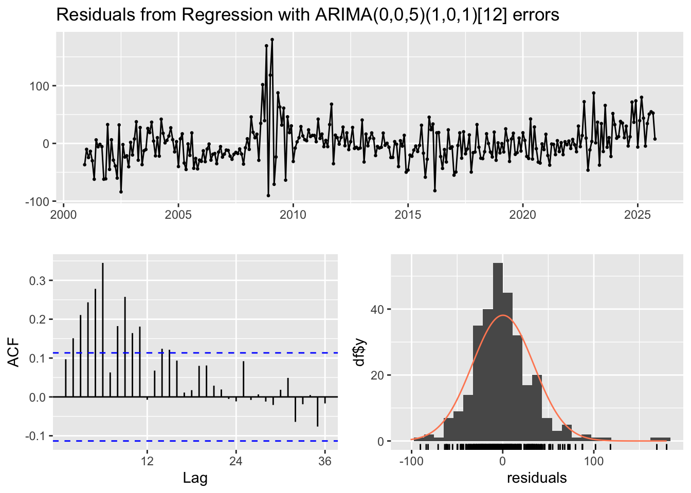
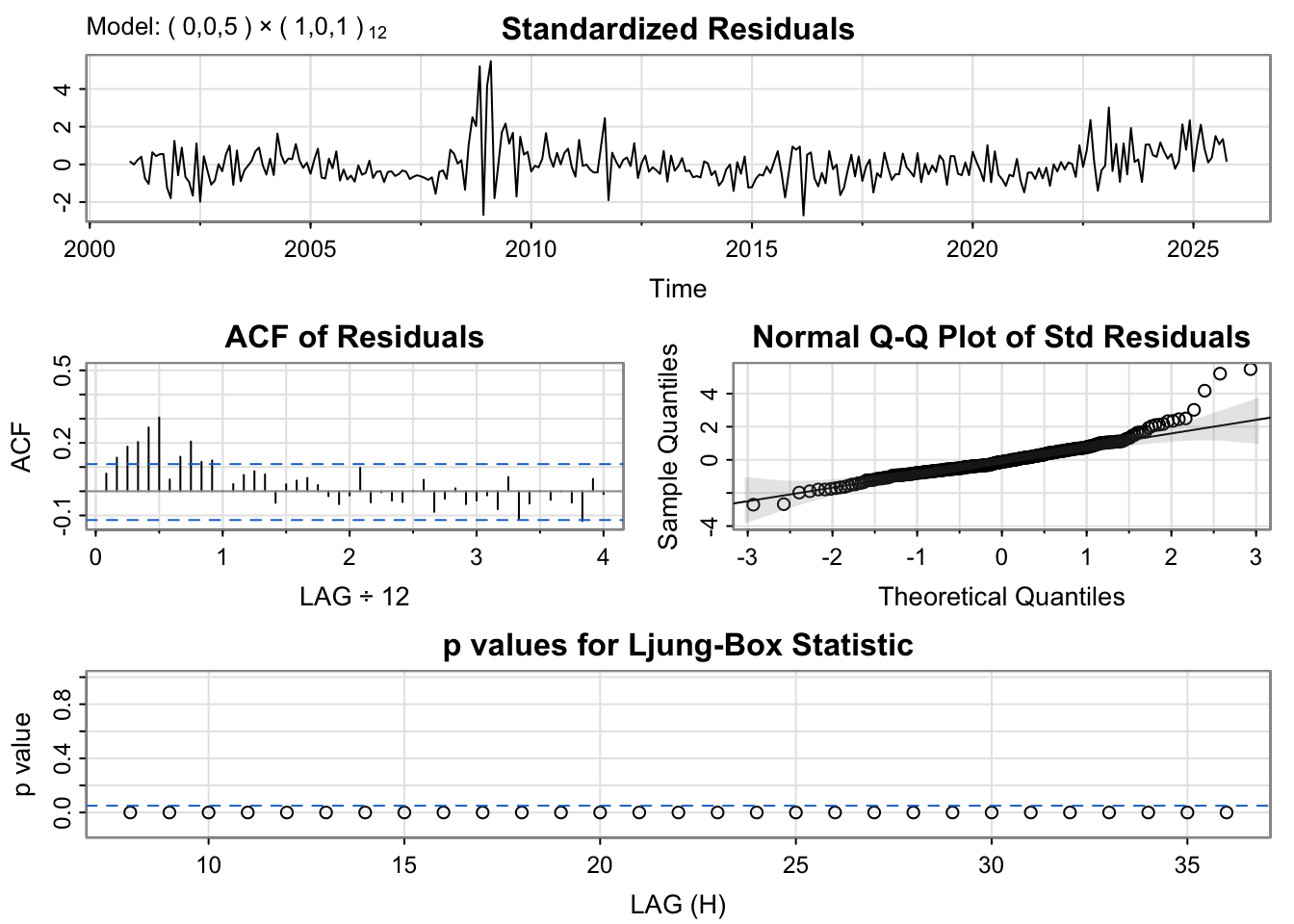
The auto.arima model exhibits noticeable autocorrelation, with a significant spike in the ACF before lag 12, suggesting the presence of remaining short-term dependence that the model has not fully captured. Additionally, the residual series displays visible fluctuations, including a pronounced period of volatility between 2008 and 2010, indicating potential structural changes or outliers during that time. These patterns imply that the model may be under-differenced or missing key components to adequately capture the temporal dynamics and seasonal structure of the data.

Code

m1<- lm(krw~ US_KR_3Y+US_KR_10Y+log_sp500_close+log_usd_index,data = df3)
summary(m1)


Call:
lm(formula = krw ~ US_KR_3Y + US_KR_10Y + log_sp500_close + log_usd_index, 
    data = df3)

Residuals:
    Min      1Q  Median      3Q     Max 
-143.28  -65.07  -13.86   45.71  448.57 

Coefficients:
                Estimate Std. Error t value Pr(>|t|)    
(Intercept)     -3085.90     245.24 -12.583  < 2e-16 ***
US_KR_3Y          -64.56      10.48  -6.160 2.38e-09 ***
US_KR_10Y          32.00      13.99   2.288   0.0229 *  
log_sp500_close    92.78      14.00   6.626 1.65e-10 ***
log_usd_index     774.29      51.50  15.036  < 2e-16 ***
---
Signif. codes:  0 '***' 0.001 '**' 0.01 '*' 0.05 '.' 0.1 ' ' 1

Residual standard error: 85.87 on 294 degrees of freedom
Multiple R-squared:  0.533, Adjusted R-squared:  0.5266 
F-statistic: 83.87 on 4 and 294 DF,  p-value: < 2.2e-16

Code

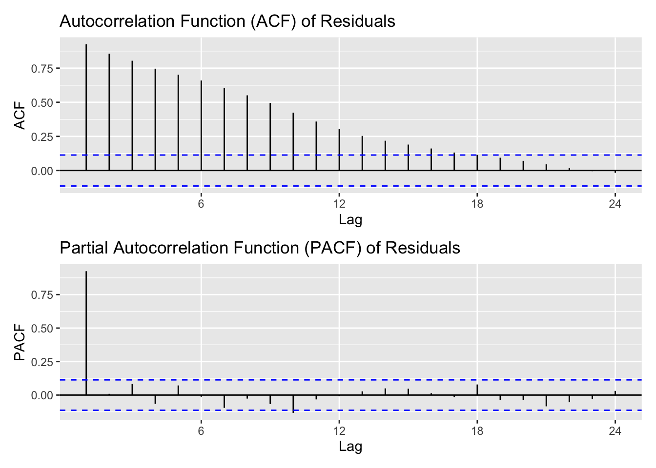
library(patchwork)
res.fit1<- ts(residuals(m1),start = c(2000,12),frequency = 12)
 
acf1<- ggAcf(res.fit1) +
  ggtitle("Autocorrelation Function (ACF) of Residuals")
pacf1<- ggPacf(res.fit1) +
  ggtitle("Partial Autocorrelation Function (PACF) of Residuals")

acf1 / pacf1

Code

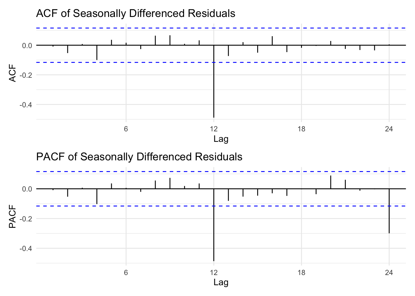
diff1<- diff(res.fit1)
seasonal_diff1<- diff(diff1,lag = 12)

diff_p1 <- ggAcf(seasonal_diff1) +
  ggtitle("ACF of Seasonally Differenced Residuals") +
  theme_minimal()

diff_p2 <- ggPacf(seasonal_diff1) +
  ggtitle("PACF of Seasonally Differenced Residuals") +
  theme_minimal()

diff_p1 /diff_p2

Code

output1 <- SARIMA.c(
  p_range = 0:2, q_range = 0:2, 
  d_range = 0:1, D_range = 0:1, 
  P_range = 1, Q_range = 0:2, 
  data = res.fit1
)


minaic <- output1[which.min(output1$AIC), ]
minbic <- output1[which.min(output1$BIC), ]

print(minaic)

   p d q P D Q      AIC      BIC    AICc
35 0 1 2 1 1 1 2840.916 2859.196 2841.13

Code

model_output_1 <- capture.output(sarima(res.fit1, 0,1,2,1,1,1,12))

Code

model_output_2 <- capture.output(sarima(res.fit1, 0,0,5,1,0,1,12))

Code

extract_model_diagnostics <- function(model_output) {
  start_line <- grep("Coefficients", model_output)  # Find where coefficients start
  end_line <- length(model_output)  # Capture till the last line
  if (length(start_line) > 0) {
    cat(model_output[start_line:end_line], sep = "\n")  # Print coefficient section
  } else {
    cat("No coefficient details found.\n")  # Handle cases where output format changes
  }
}

extract_model_diagnostics(model_output_1)

Coefficients: 
     Estimate     SE  t.value p.value
ma1   -0.0535 0.0595  -0.8997  0.3690
ma2   -0.1284 0.0626  -2.0522  0.0411
sar1  -0.0710 0.0618  -1.1498  0.2512
sma1  -1.0000 0.0596 -16.7682  0.0000

sigma^2 estimated as 1012.115 on 282 degrees of freedom 
 
AIC = 9.933272  AICc = 9.93377  BIC = 9.997188

Code

extract_model_diagnostics(model_output_2)

Coefficients: 
      Estimate     SE t.value p.value
ma1     1.0187 0.0687 14.8269  0.0000
ma2     0.8521 0.0901  9.4559  0.0000
ma3     0.7539 0.0670 11.2585  0.0000
ma4     0.5018 0.0750  6.6902  0.0000
ma5     0.2326 0.0656  3.5479  0.0005
sar1   -0.1625 0.5179 -0.3137  0.7540
sma1    0.2462 0.5044  0.4882  0.6258
xmean   1.1730 9.4233  0.1245  0.9010

sigma^2 estimated as 1233.529 on 291 degrees of freedom 
 
AIC = 10.02133  AICc = 10.02299  BIC = 10.13272

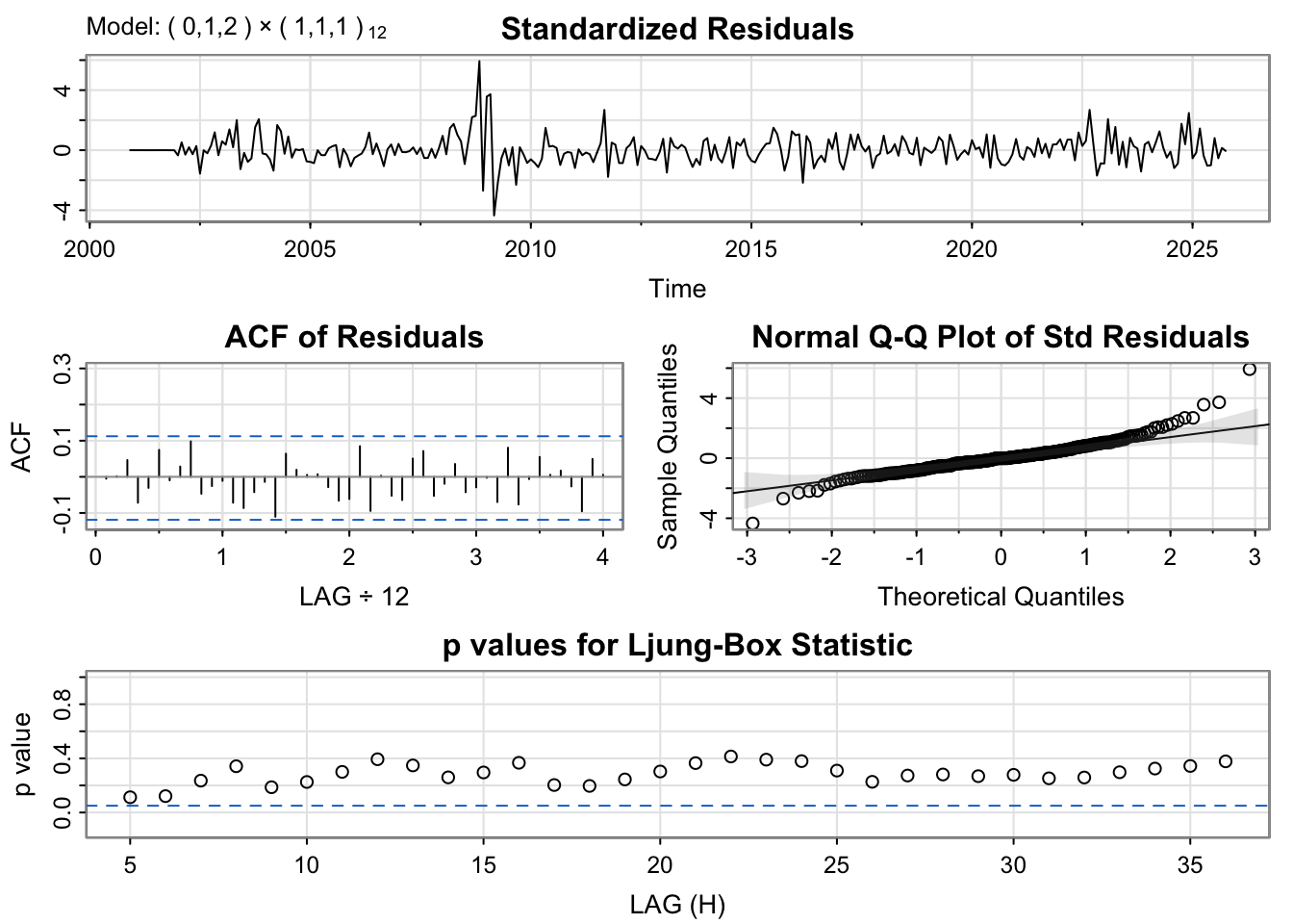
The ARIMA(0,1,2)(1,1,1)12 model produces residuals that behave much closer to white noise. The residual plot shows less obvious patterns or persistent fluctuations over time compared with the auto.arima model , indicating that both regular and seasonal differencing have successfully stabilized the series. The PACF of the residuals shows no significant spikes within the confidence bounds, suggesting that autocorrelation has been effectively removed. The Q–Q plot of standardized residuals aligns closely with the theoretical normal line, with only minor deviations at the tails. Furthermore, the Ljung–Box test p-values remain above the significance level across most lags, confirming the adequacy of the model fit. Overall, this model captures both the short-term and seasonal dynamics of the data well and provides a significant improvement over the auto.arima model.

RMSE for 12-Step Forecasts
Horizon1	RMSE_Model1	RMSE_Model2
1	75.2885	74.8425
2	75.5743	75.1145
3	75.3363	75.2164
4	74.7199	75.2525
5	74.5120	75.1724
6	74.3232	75.1111
7	74.2009	75.0476
8	74.2162	74.9261
9	74.2647	74.7324
10	74.3287	74.5284
11	74.4096	74.3075
12	74.3660	74.0836

Code

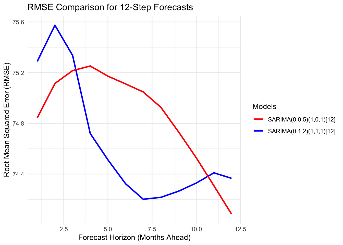
ggplot(rmse_table1, aes(x = Horizon1)) +
  geom_line(aes(y = RMSE_Model1, color = "SARIMA(0,1,2)(1,1,1)[12]"), size = 1) +
  geom_line(aes(y = RMSE_Model2, color = "SARIMA(0,0,5)(1,0,1)[12]"), size = 1) +
  labs(title = "RMSE Comparison for 12-Step Forecasts",
       x = "Forecast Horizon (Months Ahead)",
       y = "Root Mean Squared Error (RMSE)") +
  scale_color_manual(name = "Models", values = c("red", "blue")) +
  theme_minimal()

From the plots, the SARIMA(0,1,2)(1,1,1)[12] model demonstrates strong overall performance, capturing the main patterns and seasonal dynamics effectively across most of the time series. In contrast, the SARIMA(0,0,5)(1,0,1)[12] model performs slightly better in predicting values at the very beginning and end of the series, suggesting improved short-term and long-horizon accuracy. However, considering consistency and overall fit throughout the data, the SARIMA(0,1,2)(1,1,1)[12] model provides a more balanced and reliable performance. Therefore, this model is selected as the preferred choice.

Code

final_fit1<- Arima(y1,order = c(0,1,2),seasonal = list(order = c(1,1,1),period = 12),xreg = xreg1)
summary(final_fit1)

Series: y1 
Regression with ARIMA(0,1,2)(1,1,1)[12] errors 

Coefficients:
          ma1      ma2     sar1     sma1  US_KR_3Y  US_KR_10Y  log_usd_index
      -0.1410  -0.1266  -0.0513  -1.0000  -17.3951    -9.6550       883.1751
s.e.   0.0605   0.0659   0.0626   0.1413   11.5517    11.7263        77.1053
      log_sp500_close
            -219.0293
s.e.          39.0265

sigma^2 = 748.9:  log likelihood = -1368.09
AIC=2754.19   AICc=2754.84   BIC=2787.09

Training set error measures:
                   ME     RMSE      MAE       MPE    MAPE      MASE
Training set 2.461805 26.38713 19.06936 0.1743897 1.62301 0.2430716
                     ACF1
Training set -0.006297849

$$ (1+0.0513,^{{12}),(1-)(1-}{12}),y_t = -17.3951,_t -9.6550,_t +883.1751,()_t -219.0293,()_t +,(1-0.1410,,^{2),(1-1.0000,}{12}),_t.

\[ \]

\[\begin{aligned} (1 + 0.0513\,B^{12})(1 - B)(1 - B^{12})\,y_t \\[4pt] =\; -\,17.3951\,\text{US\_KR\_3Y}_t \;-\; 9.6550\,\text{US\_KR\_10Y}_t \;+\; 883.1751\,\log(\text{usd\_index})_t \;-\; 219.0293\,\log(\text{sp500\_close})_t \\[6pt] \quad+\; (1 - 0.1410\,B - 0.1266\,B^{2})(1 - 1.0000\,B^{12})\,\varepsilon_t. \end{aligned}\]

\[ \begin{alignedat}{1} &(1 + 0.0513\,B^{12})(1 - B)(1 - B^{12})\,y_t \\[4pt] &=\,-17.3951\,\text{US_KR_3Y}_t - 9.6550\,\text{US_KR_10Y}_t + 883.1751\,\log(\text{usd_index})_t - 219.0293\,\log(\text{sp500_close})_t \\[6pt] &\quad+\,(1 - 0.1410\,B - 0.1266\,B^{2})(1 - 1.0000\,B^{12})\,\varepsilon_t. \end{alignedat} \]

Code

fin_short_fit <- auto.arima(xreg1[, "US_KR_3Y"])
fshort <- forecast(fin_short_fit, h = 32) 

fin_long_fit <- auto.arima(xreg1[, "US_KR_10Y"])
flong <- forecast(fin_long_fit, h = 32)

usd_fit <- auto.arima(xreg1[, "log_usd_index"])
fusd <- forecast(usd_fit, h = 32)

sp_fit <- auto.arima(xreg1[, "log_sp500_close"])
fsp <- forecast(sp_fit, h = 32)

fxreg1 <- cbind(US_KR_3Y = fshort$mean,
                US_KR_10Y = flong$mean,
                log_usd_index = fusd$mean,
                log_sp500_close = fsp$mean)

Code

library(plotly)

fcast1 <- forecast(final_fit1, xreg = fxreg1, h = 32)

fcast_df1 <- data.frame(
  Date = as.Date(time(fcast1$mean)),
  Forecast = as.numeric(fcast1$mean),
  Lower80 = as.numeric(fcast1$lower[,1]),
  Upper80 = as.numeric(fcast1$upper[,1]),
  Lower95 = as.numeric(fcast1$lower[,2]),
  Upper95 = as.numeric(fcast1$upper[,2])
)

orig_df <- data.frame(
  Date = as.Date(time(y1)),
  Actual = as.numeric(y1)
)


plot_ly() |>
  add_lines(data = orig_df,
            x = ~Date, y = ~Actual,
            name = "Actual") |>
  add_lines(data = fcast_df1,
            x = ~Date, y = ~Forecast,
            name = "Forecast") |>
  add_ribbons(data = fcast_df1,
              x = ~Date,
              ymin = ~Lower95,
              ymax = ~Upper95,
              name = "95% CI",
              opacity = 0.2,
              showlegend = FALSE) |>
  add_ribbons(data = fcast_df1,
              x = ~Date,
              ymin = ~Lower80,
              ymax = ~Upper80,
              name = "80% CI",
              opacity = 0.3,
              showlegend = FALSE) |>
  layout(
    title = "Forecast of KRW/USD exchange spot rate for next 36 month",
    xaxis = list(title = "Year"),
    yaxis = list(title = "KRW to one USD")
  )

The forecast demonstrates a good fit, closely following the pattern of previous values. Over time, the KRW is projected to appreciate gradually, showing only minor changes and limited fluctuations.

SARIMAX model : South korea exports(vs USA) ~ VIX + US manufacturing Index + KRW/USD spot rate

data cleaning

Code

usmi<- read_csv("../data/usmi.csv")
usmi<- usmi%>% 
  rename(Date = observation_date, usm = INDPRO)%>%
  mutate(Date = ymd(Date)) %>%
  arrange(Date)

vix_monthly_m2 <- vix %>%
  mutate(year_month = floor_date(Date, "month")) %>%
  group_by(year_month) %>%
  slice_head(n = 1) %>%
  ungroup() %>%
  mutate(Date = floor_date(year_month, "month")) %>%  
  dplyr::select(Date, vix)

kor_monthly_m2 <- kr %>%
  mutate(year_month = floor_date(Date, "month")) %>%
  group_by(year_month) %>%
  slice_head(n = 1) %>%
  ungroup() %>%
  mutate(Date = floor_date(year_month, "month")) %>%  
  dplyr::select(Date, krw)

trade_exports<- trade %>%
  dplyr::select(Date, export_USD)%>%
  rename(exports = export_USD)

df4<- trade_exports%>%
  left_join(usmi,by = "Date")%>%
  left_join(vix_monthly_m2,by = "Date")%>%
  left_join(kor_monthly_m2, by = "Date")

start_year_df4  <- year(min(df4$Date))
start_month_df4 <- month(min(df4$Date))

Code

p9 <- plot_ly(df4, x = ~Date, y = ~exports, type = "scatter", mode = "lines",
              name = "South korea exports(US)") %>%
layout(yaxis = list(title = "South korea exports(US)", titlefont = list(size = 14), tickfont = list(size = 12)))

p10 <- plot_ly(df4, x = ~Date, y = ~usm, type = "scatter", mode = "lines",
              name = "US manufacturing Index") %>%
layout(yaxis = list(title = "US manufacturing Index", titlefont = list(size = 14), tickfont = list(size = 12)))

p11 <- plot_ly(df4, x = ~Date, y = ~vix, type = "scatter", mode = "lines",
              name = "VIX index") %>%
layout(yaxis = list(title = "VIX index", titlefont = list(size = 14), tickfont = list(size = 12)))

p12 <- plot_ly(df4, x = ~Date, y = ~krw, type = 'scatter', mode = 'lines',
              name = "KRW/USD spot rate") %>%
  layout(yaxis = list(title = "KRW/USD spot rate", titlefont = list(size = 14), tickfont = list(size = 12)))


subplot(p9,p12, nrows = 2, shareX = TRUE, titleY = TRUE) %>%
  layout(xaxis = list(title = "Date"))

Code

subplot(p10,p11, nrows = 2, shareX = TRUE, titleY = TRUE) %>%
  layout(xaxis = list(title = "Date"))

Code

df4.ts<- ts(df4[,c( "vix","usm","krw","exports")],start = c(1993,1),frequency = 12)
y2<- df4.ts[,"exports"]
xreg2 <- df4.ts[, !(colnames(df4.ts) %in% "exports")]
fit_auto2<- auto.arima(y2,xreg = xreg2)
summary(fit_auto2)

Series: y2 
Regression with ARIMA(0,1,1)(0,0,2)[12] errors 

Coefficients:
          ma1    sma1    sma2        vix       usm        krw
      -0.6613  0.3278  0.1766  -272.6394  97227.64  -317.6629
s.e.   0.0398  0.0544  0.0576  4246.8016  15051.92   341.1909

sigma^2 = 1.859e+11:  log likelihood = -5625.82
AIC=11265.63   AICc=11265.93   BIC=11293.41

Training set error measures:
                   ME     RMSE      MAE        MPE     MAPE      MASE      ACF1
Training set 24238.72 427248.1 307163.3 -0.3682801 7.044885 0.5508381 0.0304862

Code

checkresiduals(fit_auto2)


    Ljung-Box test

data:  Residuals from Regression with ARIMA(0,1,1)(0,0,2)[12] errors
Q* = 71.466, df = 21, p-value = 2.042e-07

Model df: 3.   Total lags used: 24

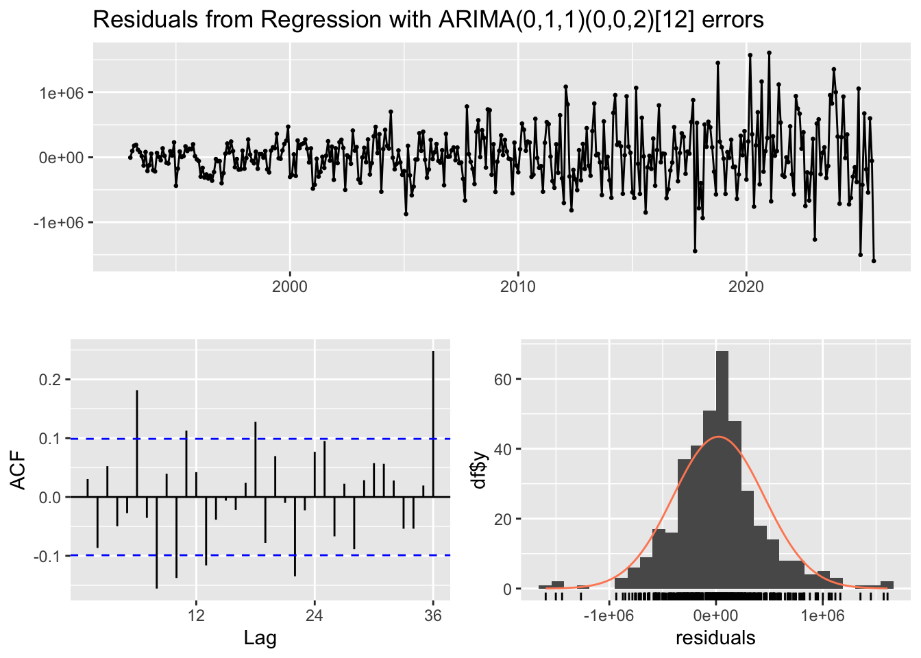
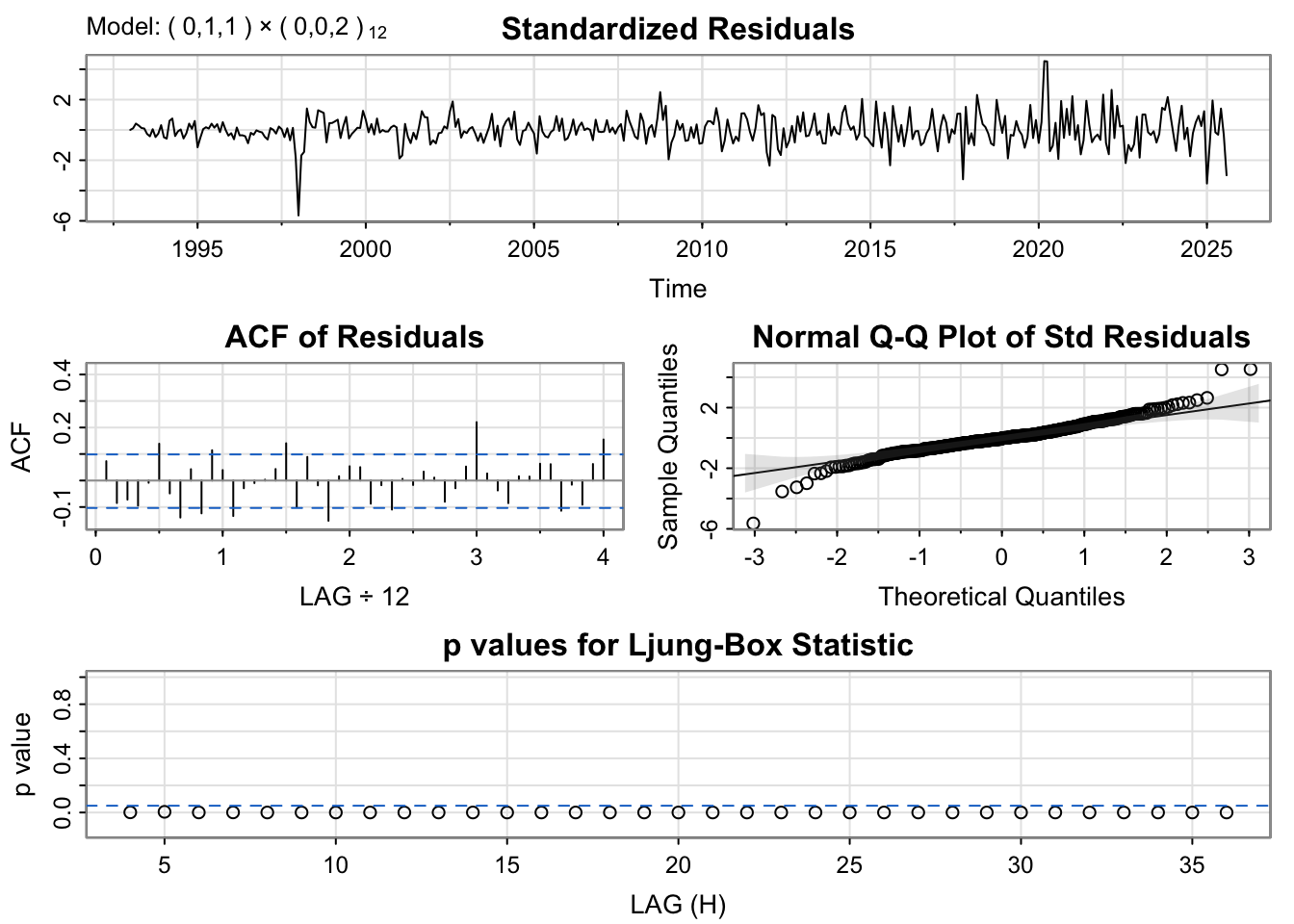
The ARIMA(0,1,1)(0,0,2)[12] model from auto.arima() yields residuals that fluctuate randomly around zero, though variability increases in recent years, indicating the fit is not perfect. The residual ACF shows only mild autocorrelation, with most lags within the 95% bounds, but a faint seasonal signal remains near lag 12. The residual histogram is approximately normal, with slight skewness driven by a few large observations.

Code

m2<- lm(exports~ usm+vix+krw, data = df4)
summary(m2)


Call:
lm(formula = exports ~ usm + vix + krw, data = df4)

Residuals:
     Min       1Q   Median       3Q      Max 
-3846667 -1306009  -267557  1170558  4378304 

Coefficients:
              Estimate Std. Error t value Pr(>|t|)    
(Intercept) -1.166e+07  7.807e+05 -14.939  < 2e-16 ***
usm          1.405e+05  9.939e+03  14.138  < 2e-16 ***
vix         -6.138e+04  1.243e+04  -4.937 1.18e-06 ***
krw          3.949e+03  6.564e+02   6.016 4.14e-09 ***
---
Signif. codes:  0 '***' 0.001 '**' 0.01 '*' 0.05 '.' 0.1 ' ' 1

Residual standard error: 1639000 on 388 degrees of freedom
Multiple R-squared:  0.5771,    Adjusted R-squared:  0.5738 
F-statistic: 176.5 on 3 and 388 DF,  p-value: < 2.2e-16

Code

library(patchwork)
res.fit2<- ts(residuals(m2),start = c(1993,1),frequency = 12)
 
acf2<- ggAcf(res.fit2) +
  ggtitle("Autocorrelation Function (ACF) of Residuals")
pacf2<- ggPacf(res.fit2) +
  ggtitle("Partial Autocorrelation Function (PACF) of Residuals")

acf2 / pacf2

Code

diff2<- diff(res.fit2)
seasonal_diff2<- diff(diff2,lag = 12)

diff_p3 <- ggAcf(seasonal_diff2) +
  ggtitle("ACF of Seasonally Differenced Residuals") +
  theme_minimal()

diff_p4 <- ggPacf(seasonal_diff2) +
  ggtitle("PACF of Seasonally Differenced Residuals") +
  theme_minimal()

diff_p3 /diff_p4

Code

output2 <- SARIMA.c(
  p_range = 0:3, q_range = 0:3, 
  d_range = 1, D_range = 1, 
  P_range = 0:1, Q_range = 0:1, 
  data = res.fit2
)


minaic <- output2[which.min(output2$AIC), ]
minbic <- output2[which.min(output2$BIC), ]

print(minaic)

   p d q P D Q      AIC   BIC     AICc
64 3 1 3 1 1 1 11054.56 11090 11055.05

Code

print(minbic)

  p d q P D Q      AIC      BIC     AICc
6 0 1 1 0 1 1 11067.37 11079.19 11067.44

Code

model_output_3 <- capture.output(sarima(res.fit2, 3,1,3,1,1,1,12))

Code

model_output_4 <- capture.output(sarima(res.fit2, 0,1,1,0,1,1,12))

Code

model_output_5 <- capture.output(sarima(res.fit2, 0,1,1,0,0,2,12))

Code

extract_model_diagnostics <- function(model_output) {
  start_line <- grep("Coefficients", model_output)  # Find where coefficients start
  end_line <- length(model_output)  # Capture till the last line
  if (length(start_line) > 0) {
    cat(model_output[start_line:end_line], sep = "\n")  # Print coefficient section
  } else {
    cat("No coefficient details found.\n")  # Handle cases where output format changes
  }
}

extract_model_diagnostics(model_output_3)

Coefficients: 
     Estimate     SE  t.value p.value
ar1   -0.7264 0.1336  -5.4372  0.0000
ar2   -0.6606 0.1726  -3.8272  0.0002
ar3    0.2760 0.1270   2.1727  0.0304
ma1    0.2731 0.1184   2.3054  0.0217
ma2    0.3130 0.1246   2.5111  0.0125
ma3   -0.6248 0.0889  -7.0254  0.0000
sar1  -0.1804 0.0676  -2.6684  0.0080
sma1  -0.8364 0.0403 -20.7679  0.0000

sigma^2 estimated as 246828438646 on 371 degrees of freedom 
 
AIC = 29.1677  AICc = 29.16873  BIC = 29.2612

Code

extract_model_diagnostics(model_output_4)

Coefficients: 
     Estimate     SE  t.value p.value
ma1   -0.4833 0.0500  -9.6756       0
sma1  -0.8691 0.0277 -31.3438       0

sigma^2 estimated as 2.64877e+11 on 377 degrees of freedom 
 
AIC = 29.20151  AICc = 29.2016  BIC = 29.23268

Code

extract_model_diagnostics(model_output_5)

Coefficients: 
          Estimate         SE t.value p.value
ma1        -0.5181     0.0536 -9.6671  0.0000
sma1        0.1351     0.0525  2.5738  0.0104
sma2        0.2083     0.0492  4.2301  0.0000
constant 1817.6271 18188.1618  0.0999  0.9204

sigma^2 estimated as 314616300440 on 387 degrees of freedom 
 
AIC = 29.34198  AICc = 29.34225  BIC = 29.39273

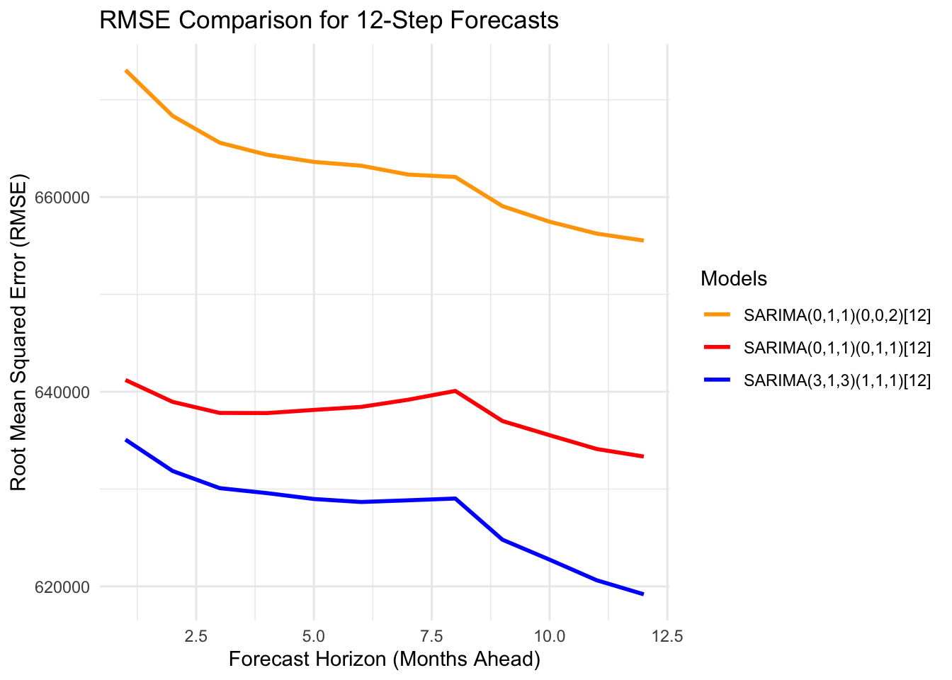
All three models display similar residual patterns, characterized by random fluctuations around zero with a few noticeable outlier spikes. The ACF plots of the residuals also show comparable behavior across models; however, the ARIMA(3,1,3)(1,1,1)[12] model performs slightly better, as its autocorrelations remain within the significance bounds across most lags. The normal Q–Q plots indicate that all models exhibit similar residual distributions, with deviations at the tails suggesting the presence of non-normality often observed in time series data. Although the Ljung–Box test results indicate that none of the models fully satisfy the white noise assumption—since most p-values fall below the significance threshold—the ARIMA(0,1,1)(0,1,1)[12] model appears to offer a marginally better fit compared to the others.

RMSE for 12-Step Forecasts
Horizon1	RMSE_Model1	RMSE_Model2	RMSE_Model3
1	635078.8	641208.0	673054.1
2	631856.4	638958.8	668345.2
3	630093.2	637819.6	665584.1
4	629582.7	637805.9	664351.6
5	628977.1	638130.8	663611.2
6	628669.7	638440.3	663223.7
7	628843.3	639176.5	662312.4
8	629025.6	640080.4	662063.7
9	624796.7	636988.8	659068.0
10	622747.3	635535.4	657468.8
11	620629.7	634116.4	656244.0
12	619185.3	633339.6	655531.3

Code

ggplot(rmse_table1, aes(x = Horizon1)) +
  geom_line(aes(y = RMSE_Model1, color = "SARIMA(3,1,3)(1,1,1)[12]"), size = 1) +
  geom_line(aes(y = RMSE_Model2, color = "SARIMA(0,1,1)(0,1,1)[12]"), size = 1) +
  geom_line(aes(y = RMSE_Model3, color = "SARIMA(0,1,1)(0,0,2)[12]"), size = 1) +
  labs(title = "RMSE Comparison for 12-Step Forecasts",
       x = "Forecast Horizon (Months Ahead)",
       y = "Root Mean Squared Error (RMSE)") +
  scale_color_manual(name = "Models", values = c("orange","red", "blue")) +
  theme_minimal()

From the plot, SARIMA(3,1,3)(1,1,1)[12] performs better than other models, so SARIMA(3,1,3)(1,1,1)[12] model is best model.

Code

final_fit2<- Arima(y2,order = c(3,1,3),seasonal = list(order = c(1,1,1),period = 12),xreg = xreg2)
summary(final_fit2)

Series: y2 
Regression with ARIMA(3,1,3)(1,1,1)[12] errors 

Coefficients:
         ar1      ar2      ar3     ma1     ma2      ma3     sar1     sma1
      -1.216  -1.0579  -0.0649  0.6024  0.3140  -0.5152  -0.0829  -0.8007
s.e.   0.102   0.1152   0.0985  0.0906  0.0949   0.0849   0.0662   0.0417
            vix       usm        krw
      -6911.305  97511.41  -220.2439
s.e.   3920.370  14375.69   326.3332

sigma^2 = 1.433e+11:  log likelihood = -5407.54
AIC=10839.08   AICc=10839.93   BIC=10886.33

Training set error measures:
                   ME     RMSE      MAE           MPE     MAPE      MASE
Training set 17649.08 366715.5 258171.3 -0.0009533994 5.717243 0.4629803
                     ACF1
Training set -0.002233551

\[ \begin{aligned} \bigl(1 + 1.216\,B + 1.0579\,B^{2} + 0.0649\,B^{3}\bigr) \bigl(1 + 0.0829\,B^{12}\bigr) w_t \\[4pt] =\; -\,6911.305\,\mathrm{vix}_t \;+\; 97{,}511.41\,\mathrm{usm}_t \;-\; 220.2439\,\mathrm{krw}_t \\[6pt] \quad+\; \bigl(1 + 0.6024\,B + 0.3140\,B^{2} - 0.5152\,B^{3}\bigr) \bigl(1 - 0.8007\,B^{12}\bigr)\varepsilon_t, \\[6pt] \varepsilon_t &\sim \mathcal{N}(0, \sigma^2). \end{aligned} \]

Code

usm_fit <- auto.arima(xreg2[, "usm"])
fusm <- forecast(usm_fit, h = 48) 

vix_fit <- auto.arima(xreg2[, "vix"])
fvix <- forecast(vix_fit, h = 48)

krw_fit <- auto.arima(xreg2[, "krw"])
fkrw <- forecast(krw_fit, h = 48)


fxreg2 <- cbind(vix = fvix$mean,
                usm = fusm$mean,
                krw = fkrw$mean)

Code

library(plotly)

fcast2 <- forecast(final_fit2, xreg = fxreg2, h = 48)

orig_df <- data.frame(
  Date   = as.Date(as.yearmon(time(y2))),
  Actual = as.numeric(y2)
)

fcast_df2 <- data.frame(
  Date     = as.Date(as.yearmon(time(fcast2$mean))),
  Forecast = as.numeric(fcast2$mean),
  Lower80  = as.numeric(fcast2$lower[,1]),
  Upper80  = as.numeric(fcast2$upper[,1]),
  Lower95  = as.numeric(fcast2$lower[,2]),
  Upper95  = as.numeric(fcast2$upper[,2])
)


plot_ly() |>
  add_lines(data = orig_df,
            x = ~Date, y = ~Actual,
            name = "Actual") |>
  add_lines(data = fcast_df2,
            x = ~Date, y = ~Forecast,
            name = "Forecast") |>
  add_ribbons(data = fcast_df2,
              x = ~Date,
              ymin = ~Lower95,
              ymax = ~Upper95,
              name = "95% CI",
              opacity = 0.2,
              showlegend = FALSE) |>
  add_ribbons(data = fcast_df2,
              x = ~Date,
              ymin = ~Lower80,
              ymax = ~Upper80,
              name = "80% CI",
              opacity = 0.3,
              showlegend = FALSE) |>
  layout(
    title = "Forecast of South korea export to US for next 48 month",
    xaxis = list(title = "Year"),
    yaxis = list(title = "thousand USD")
  )

The forecast demonstrates a strong fit, effectively capturing the pattern of historical values. Over the projection horizon, Korea’s exports in U.S. dollars are expected to exhibit an overall upward trend, although short-term monthly fluctuations are likely to continue.

Conclusion

The model-fitting process was satisfactory and produced reasonable forecasts across the four specifications. While the results are encouraging, no model is perfect, and additional refinement would further strengthen the analysis. Because macroeconomic and financial outcomes are shaped by many interacting forces, any empirical model will have limitations. Important drivers can be difficult to observe or may change over time, so the forecasts should be interpreted with appropriate caution.

Even so, the multivariate analysis yielded meaningful insights that align with established economic relationships. None of the models produced results that ran counter to typical behavior. Instead, the estimated effects were broadly consistent with how key variables usually interact—through risk sentiment, interest-rate differentials, exchange-rate channels, and demand conditions—making the forecast interpretations economically credible.

For the VAR linking U.S. and Korean equities (S&P 500, VIX, U.S. yield spread, and KOSPI), the forecast plot indicates firmer U.S. equity conditions and wider yield spreads alongside a softer KOSPI. This is consistent with the discount-rate and risk-transmission channels: tighter U.S. financial conditions and stronger dollar dynamics raise discount rates, elevate global risk premia, and tend to weigh on KRW-sensitive Korean equities.

For the VAR examining rate pass-through to Seoul housing (U.S. 10Y, Korea 10Y, and Seoul HPI), the forecast shows gradually easing long-term yields and a firmer housing index. The opposite co-movement is exactly what the affordability channel predicts: declines in global and domestic long rates filter into borrowing costs with lags, supporting housing demand and prices over time. For the SARIMAX model of USD/KRW (with rate differentials, U.S. equities/risk, and a broad dollar factor as exogenous drivers), the forecast suggests a mild KRW appreciation path with limited volatility. This reflects the background mechanism in which narrower rate differentials, improved risk sentiment, and a cooler broad dollar typically favor KRW strength, while the ARIMA component absorbs serial dependence in the exchange rate.

For the SARIMAX model of Korea’s exports to the United States (driven by U.S. demand, the exchange rate, and risk conditions), the forecast points to an upward trend tempered by month-to-month noise. Stronger U.S. manufacturing activity pulls Korean exports higher, while exchange-rate valuation and risk/financing conditions modulate near-term fluctuations—patterns commonly observed for dollar-invoicing exporters.

Looking ahead, the models can be enhanced with deeper diagnostics, and the addition of relevant external variables such as global demand proxies beyond the U.S., commodity prices, and credit conditions. Taken together, the four models provide a coherent basis for narrative forecasting while highlighting clear avenues for continued improvement.

Reference

Kim, S. Do s&p 500 and KOSPI move together? A functional regression approach. KDI Economic Policy Review (2010).

Lee, C. The time-varying effect of interest rates on housing prices. Land (2022).

Min, C.-H. Time-varying analysis of housing prices in korea and the u.s. International Journal of Labor Economics (2024).

Yoon, D. R. What determines the exchange rate of the korean won? (2019).

Masujima, M. The shifting drivers of exchange rates. (2018).

Son, M. et al. Dominant currency pricing: Evidence from korean exports. (2023).