The focus of this section is on building financial time series models, specifically for the KOSPI Index and the KRW/USD spot exchange rate. The aim of this project is to examine the influence of the United States on the South Korean economy. More specifically, in this section the goal is to examine how dollar exchange rate risk affects the Korean economy.
The KOSPI Index serves as the main equity index for the Korean financial market and visibly reflects the overall state of Korea’s economy. The exchange rate is a very unique financial asset: it behaves like an equity asset, but is also closely related to the policy rate. Because the exchange rate reflects the value of a currency, governments use it as one of the indicators when deciding their policy rate. Since one variable (the KOSPI) reflects the pure market condition and the other (the exchange rate) contains information about currency value and monetary policy, together they form a strong set of indicators for this project.
The previous section (on multivariate time series models) focused on interactions among variables and their effects. This section instead focuses on the volatility of the variables. As financial assets, the KOSPI Index and the exchange rate are heavily influenced by various factors, which leads to volatility clustering: periods of high volatility tend to be followed by similarly turbulent periods, while calm periods also cluster together. In other words, volatility changes over time depending on past shocks and past variance. Therefore, the focus of this section is to examine volatility and its patterns by applying ARCH/GARCH models. Using these models, the aim is to understand how the volatility of the KOSPI Index and the KRW/USD exchange rate has evolved over time and how major economic crises have affected them. From this analysis, it will be possible to gain deeper intuition about how the value of the Korean won against the U.S. dollar impacts the Korean economy, particularly from a risk management perspective. For further research, the aim is to derive implications for constructing investment portfolios for effective risk management.
As discussed in the univariate and multivariate time series model sections, the log transformation performed well for the KOSPI data, so it was applied to the KOSPI closing prices. The first plot is a candlestick chart of the KOSPI Index, and the second is the log-transformed KOSPI data. It is evident that applying the log transformation reduces variability.
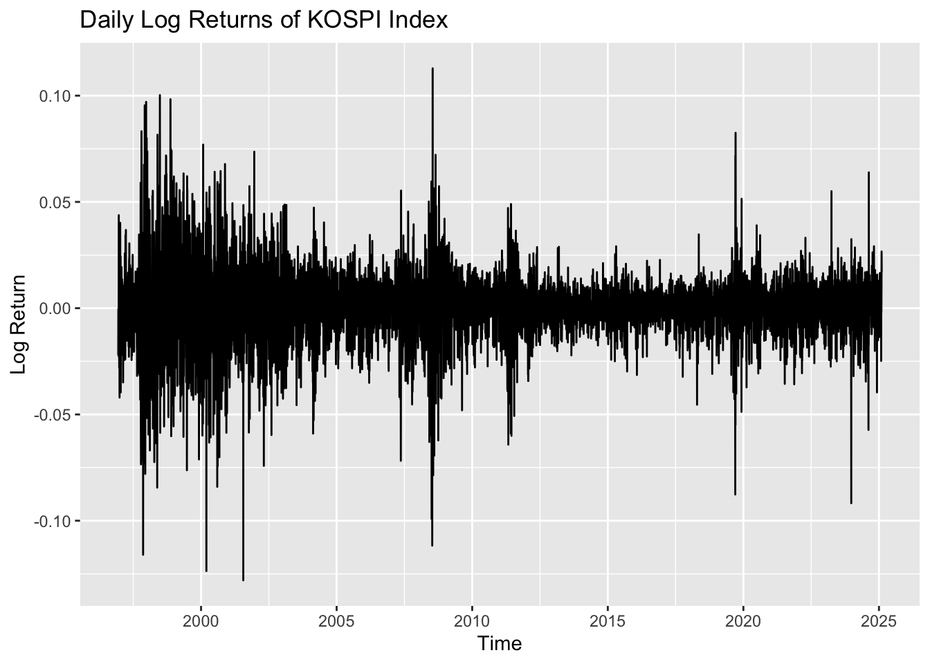
The third plot shows the log returns of the KOSPI Index. In this plot, volatility clustering is clearly observed: for most periods, the values are centered near zero, but in certain periods the series exhibits high volatility before returning to calmer behavior. This suggests that the data are potentially appropriate for modeling with the ARCH/GARCH family of models.
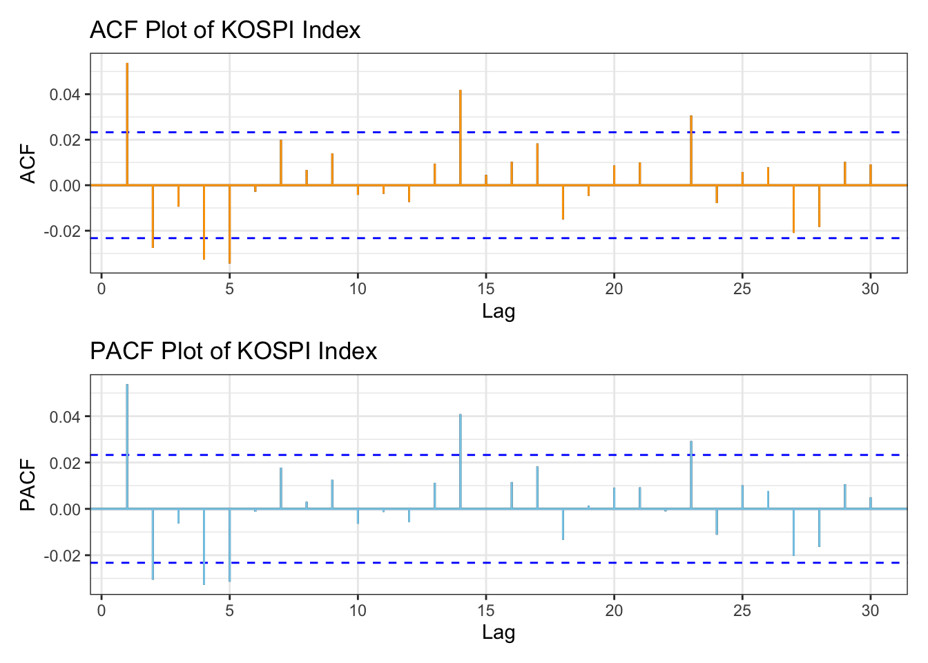
library(patchwork)kospi_acf <-ggAcf(kospi_return,lag.max =30)+ggtitle("ACF Plot of KOSPI Index") +theme_bw() +geom_segment(lineend ="butt", color ="orange") +geom_hline(yintercept =0, color ="orange") kospi_pacf <-ggPacf(kospi_return,lag.max =30)+ggtitle("PACF Plot of KOSPI Index") +theme_bw()+geom_segment(lineend ="butt", color ="skyblue") +geom_hline(yintercept =0, color ="skyblue") kospi_acf/kospi_pacf
From the plots, KOSPI Index data performs well in terms of autocorrelation by applying log transformation, However there are still some lag points showing autocorrelation.
Code
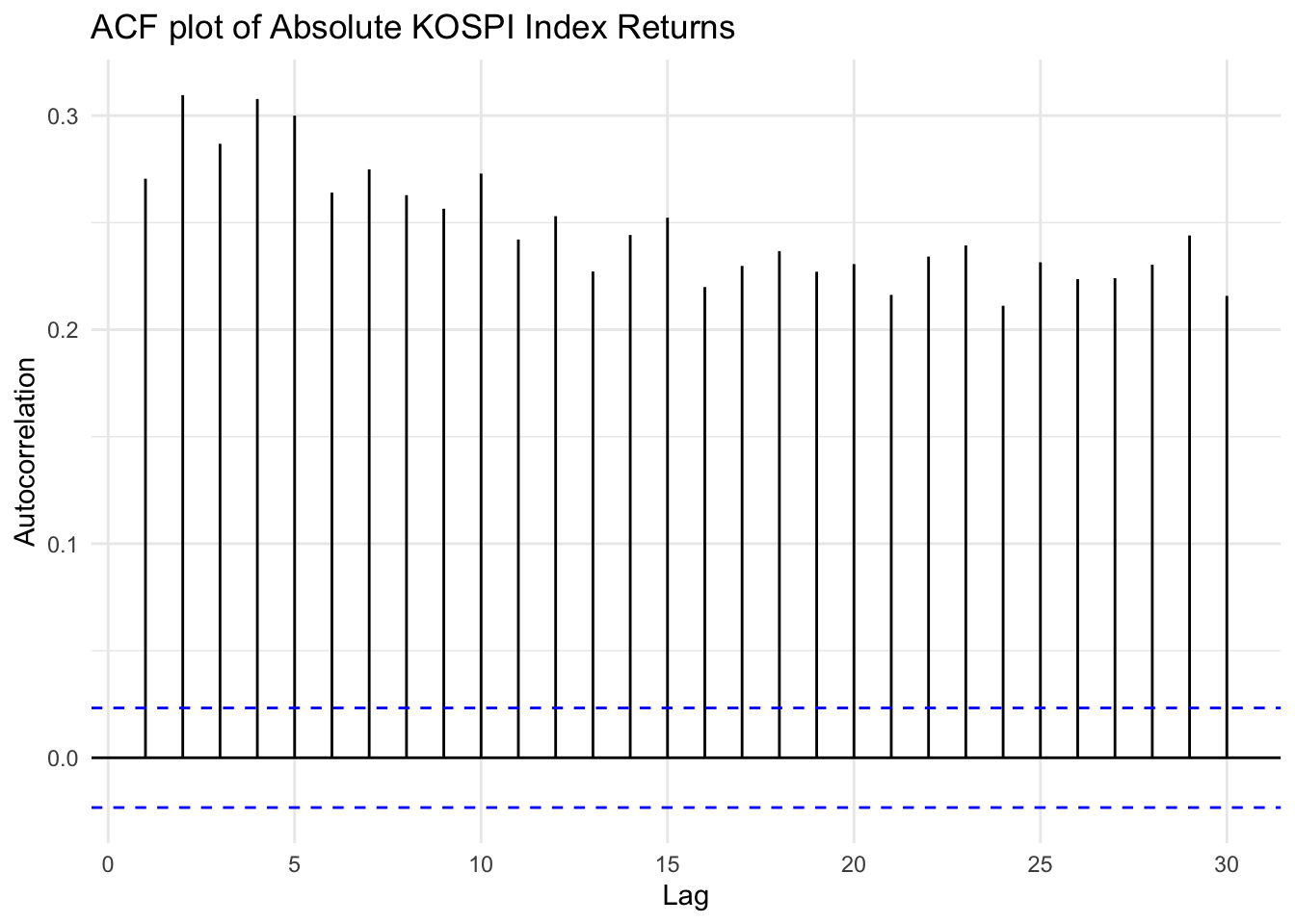
ggAcf(abs(kospi_return), lag.max =30) +ggtitle("ACF plot of Absolute KOSPI Index Returns") +xlab("Lag") +ylab("Autocorrelation") +theme_minimal()
Code
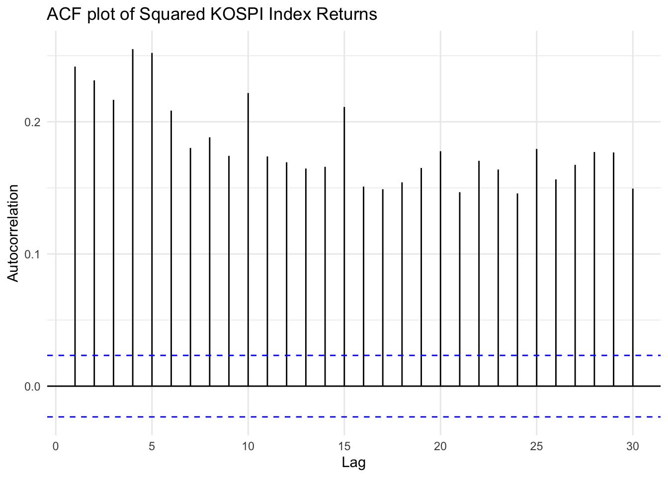
ggAcf(kospi_return^2, lag.max =30) +ggtitle("ACF plot of Squared KOSPI Index Returns") +xlab("Lag") +ylab("Autocorrelation") +theme_minimal()
Code
# Load required packagelibrary(FinTS)# Perform ARCH LM Test on Bitcoin returnsarch_test_result <-ArchTest(kospi_return, lags =1, demean =TRUE)# Print resultsprint(arch_test_result)
p-vlaue is smaller than 0.05(default criterion), indicating rejecting null hypothesis, concluding strong evidence for the presence of ARCH(1) effects in the data.
Two plots for applying absolute value and squaring to KOSPI Index shows significant autocorrelation throughout multiple lags, compare to log return. This implies that the returns are not independently and identically distributed, and gives evidence for need to apply conditional variance models such as ARCH or GARCH to capture the underlying time-varying volatility structure.
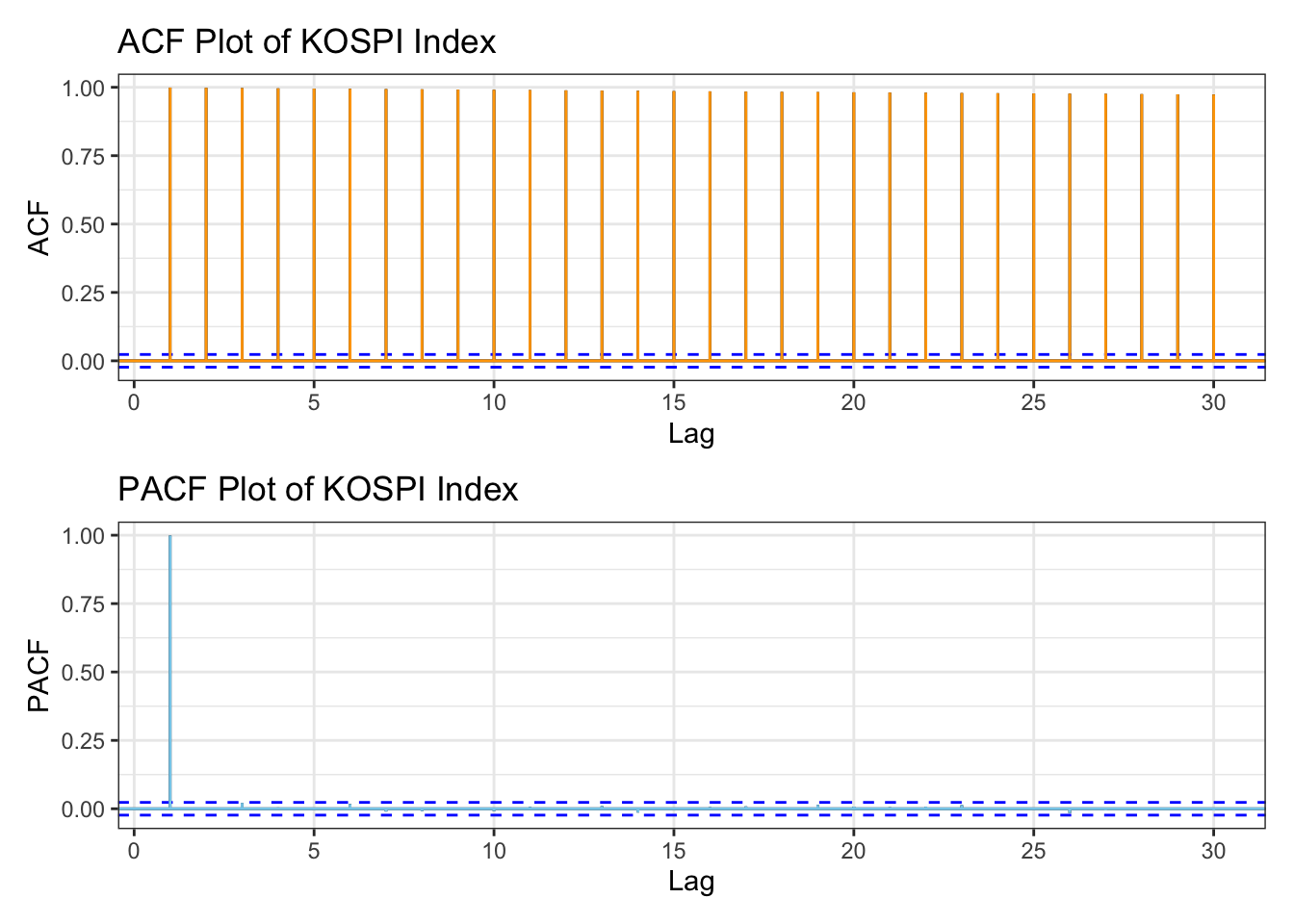
library(patchwork)kospi_acf <-ggAcf(kospi_ts,lag.max =30)+ggtitle("ACF Plot of KOSPI Index") +theme_bw() +geom_segment(lineend ="butt", color ="orange") +geom_hline(yintercept =0, color ="orange") kospi_pacf <-ggPacf(kospi_ts,lag.max =30)+ggtitle("PACF Plot of KOSPI Index") +theme_bw()+geom_segment(lineend ="butt", color ="skyblue") +geom_hline(yintercept =0, color ="skyblue") kospi_acf/kospi_pacf
Code
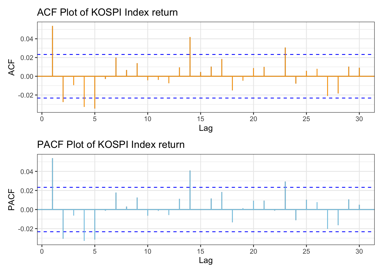
kospi_acf_log <-ggAcf(kospi_return,lag.max =30)+ggtitle("ACF Plot of KOSPI Index return") +theme_bw() +geom_segment(lineend ="butt", color ="orange") +geom_hline(yintercept =0, color ="orange") kospi_pacf_log <-ggPacf(kospi_return,lag.max =30)+ggtitle("PACF Plot of KOSPI Index return") +theme_bw()+geom_segment(lineend ="butt", color ="skyblue") +geom_hline(yintercept =0, color ="skyblue") kospi_acf_log/kospi_pacf_log
The ACF plot shows significant autocorrelation across several lags. In the PACF plot, there is a strong autocorrelation at lag 1, followed by a sharp drop, indicating almost no autocorrelation after lag 1. These plots suggest the presence of dependencies between past and current price movements, and that the series is stationary.
For the KOSPI index returns, the ACF and PACF plots show that most lags lie within the significance bounds; however, there are a few spikes at certain lags, such as lag 5. For manual model selection, a search range from 0 to 5 therefore seems appropriate.
Both plots exhibit similar patterns, indicating that conditional heteroskedasticity is present in the return series. Thus, applying models from the ARCH/GARCH family is appropriate.
Coefficients:
         Estimate     SE t.value p.value
ar1       -0.1215 0.3386 -0.3588  0.7198
ar2       -0.2424    NaN     NaN     NaN
ar3       -0.3047 0.1665 -1.8306  0.0672
ar4       -0.3587    NaN     NaN     NaN
ar5       -0.4073 0.3252 -1.2525  0.2104
ma1        0.1737 0.3328  0.5219  0.6018
ma2        0.2205    NaN     NaN     NaN
ma3        0.3098 0.1597  1.9394  0.0525
ma4        0.3444    NaN     NaN     NaN
ma5        0.3908 0.3151  1.2405  0.2148
constant   0.0002 0.0002  1.1625  0.2451

sigma^2 estimated as 0.0002647793 on 7085 degrees of freedom

AIC = -5.395351  AICc = -5.395345  BIC = -5.383737
Three models were tested: ARIMA(0,1,1), ARIMA(5,1,5), and ARIMA(2,1,2).
From the model diagnostics for these three candidates, the results are not fully satisfactory. Therefore, to decide which model to use, I compare their AIC and BIC values as well as the significance of the coefficients. Based on these criteria, I choose the ARIMA(0,1,1) model, since it has the lowest BIC value.
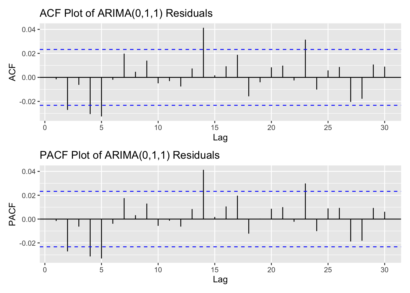
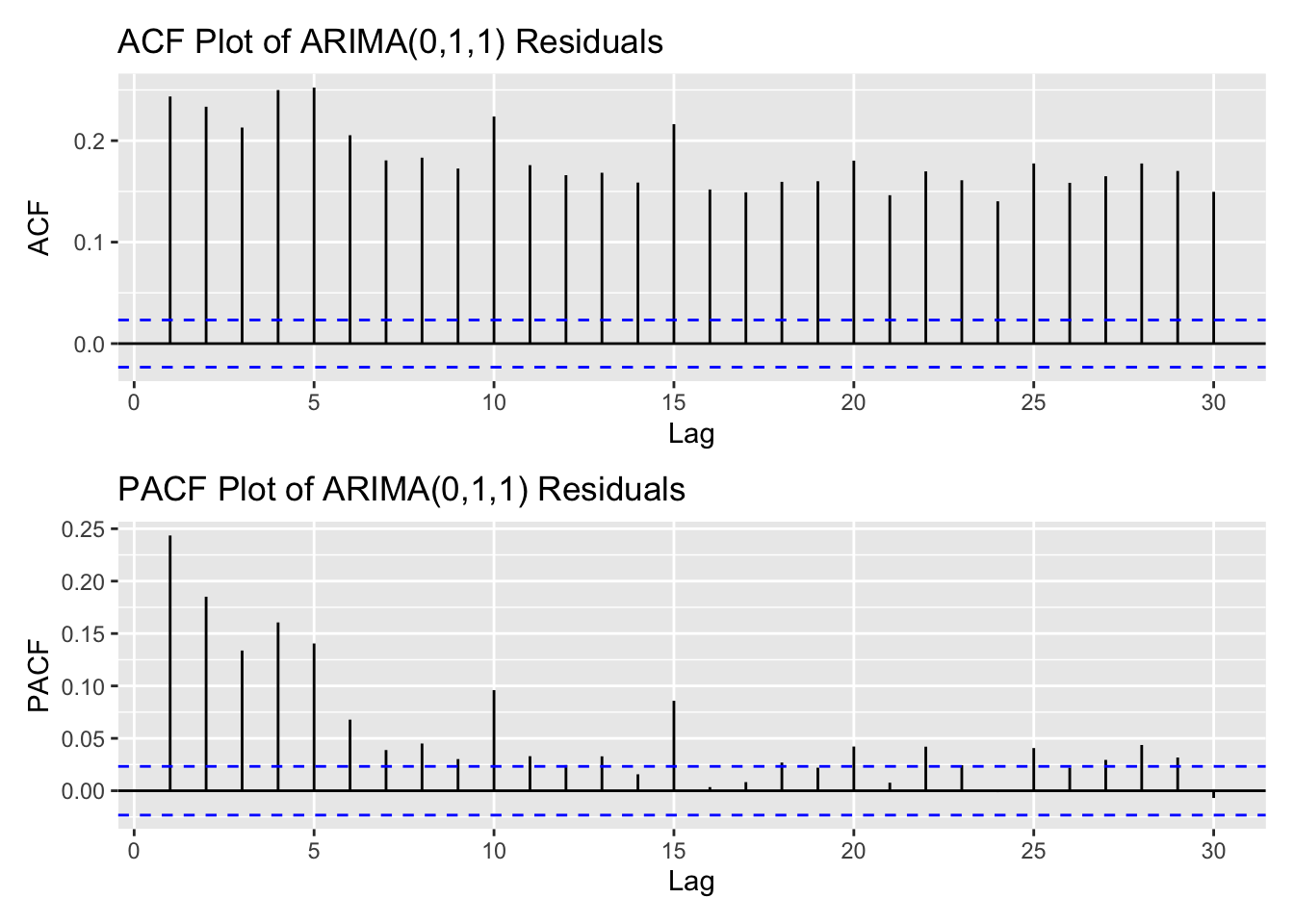
arima_fit1 <-Arima(log(kospi_ts), order =c(0,1,1), include.drift =TRUE)res_arima1<-residuals(arima_fit1)kospi_res_acf <-ggAcf(res_arima1,lag.max =30)+ggtitle("ACF Plot of ARIMA(0,1,1) Residuals") kospi_res_pacf <-ggPacf(res_arima1,lag.max =30)+ggtitle("PACF Plot of ARIMA(0,1,1) Residuals") kospi_res_acf/kospi_res_pacf
Code
arima_fit1 <-Arima(log(kospi_ts), order =c(0,1,1), include.drift =TRUE)res_arima1<-residuals(arima_fit1)kospi_res_acf <-ggAcf(res_arima1^2,lag.max =30)+ggtitle("ACF Plot of ARIMA(0,1,1) Residuals") kospi_res_pacf <-ggPacf(res_arima1^2,lag.max =30)+ggtitle("PACF Plot of ARIMA(0,1,1) Residuals") kospi_res_acf/kospi_res_pacf
From the ACF and PACF plots of the residuals and squared residuals for the ARIMA(0,1,1) model, the ACF of the squared residuals shows noticeable spikes up to lag 5, followed by a gradual decline. This suggests the presence of an ARCH effect, indicating time-varying volatility in the data. Based on these plots, an appropriate range for manual model search is p,q both in 0:5 range.
Code
library(tseries)library(knitr)library(kableExtra)# Initialize list to store models and track p, qmodels <-list()pq_combinations <-data.frame(p =integer(), q =integer(), AIC =numeric())cc <-1# Fit GARCH(p, q) models for p = 1:7 and q = 1:7for (p in0:5) {for (q in0:5) { fit <-tryCatch(garch(res_arima1, order =c(q, p), trace =FALSE),error =function(e) NULL )if (!is.null(fit)) { models[[cc]] <- fit pq_combinations <-rbind( pq_combinations,data.frame(p = p, q = q, AIC =AIC(fit)) ) cc <- cc +1 } }}# Round AIC for presentationpq_combinations$AIC <-round(pq_combinations$AIC, 3)# Identify row with minimum AIChighlight_row <-which.min(pq_combinations$AIC)# Create formatted tablepq_combinations %>%kable(caption ="AIC Comparison for GARCH(p, q) Models",col.names =c("ARCH Order (p)", "GARCH Order (q)", "AIC"),align =c("c", "c", "c"),booktabs =TRUE ) %>%kable_styling(full_width =FALSE,position ="center",bootstrap_options =c("striped", "hover", "condensed") ) %>%row_spec(highlight_row, bold =TRUE, background ="#FFF59D")
AIC Comparison for GARCH(p, q) Models
ARCH Order (p)
GARCH Order (q)
AIC
0
1
-38279.50
0
2
-38272.96
0
3
-38264.56
0
4
-38258.07
0
5
-38250.50
1
0
-39310.73
1
1
-41741.28
1
2
-41735.45
1
3
-41720.48
1
4
-41681.63
1
5
-41646.06
2
0
-40159.82
2
1
-41735.07
2
2
-41733.12
2
3
-41754.15
2
4
-41727.00
2
5
-41719.92
3
0
-40581.16
3
1
-41630.17
3
2
-41737.87
3
3
-41702.15
3
4
-41691.90
3
5
-41706.77
4
0
-40893.89
4
1
-41473.17
4
2
-41587.73
4
3
-41620.88
4
4
-41664.12
4
5
-41722.97
5
0
-41103.55
5
1
-41552.01
5
2
-41585.24
5
3
-41599.98
5
4
-41613.78
5
5
-41712.33
Code
cat("\nSummary for GARCH(2,3):\n")
Summary for GARCH(2,3):
Code
garch_model <-garchFit(~garch(2, 3), data = res_arima1, trace =FALSE)summary(garch_model)
Title:
 GARCH Modelling

Call:
 garchFit(formula = ~garch(2, 3), data = res_arima1, trace = FALSE)

Mean and Variance Equation:
 data ~ garch(2, 3)
<environment: 0x1374353c0>
 [data = res_arima1]

Conditional Distribution:
 norm

Coefficient(s):
        mu       omega      alpha1      alpha2       beta1       beta2
1.0481e-05  2.3678e-06  9.1156e-02  6.7207e-02  4.1120e-01  1.0000e-08
     beta3
4.2549e-01

Std. Errors:
 based on Hessian

Error Analysis:
        Estimate  Std. Error  t value Pr(>|t|)
mu     1.048e-05   1.234e-04    0.085   0.9323
omega  2.368e-06   5.141e-07    4.606 4.11e-06 ***
alpha1 9.116e-02   1.291e-02    7.060 1.66e-12 ***
alpha2 6.721e-02   2.354e-02    2.855   0.0043 **
beta1  4.112e-01   2.247e-01    1.830   0.0672 .
beta2  1.000e-08   3.332e-01    0.000   1.0000
beta3  4.255e-01   1.594e-01    2.670   0.0076 **
---
Signif. codes:  0 '***' 0.001 '**' 0.01 '*' 0.05 '.' 0.1 ' ' 1

Log Likelihood:
 20881.73    normalized:  2.942332

Description:
 Thu Nov 20 15:29:25 2025 by user:


Standardised Residuals Tests:
                                  Statistic   p-Value
 Jarque-Bera Test   R    Chi^2  1043.423936 0.0000000
 Shapiro-Wilk Test  R    W               NA        NA
 Ljung-Box Test     R    Q(10)     8.752495 0.5557429
 Ljung-Box Test     R    Q(15)    11.756310 0.6973730
 Ljung-Box Test     R    Q(20)    16.536223 0.6828505
 Ljung-Box Test     R^2  Q(10)     3.720897 0.9590607
 Ljung-Box Test     R^2  Q(15)    10.652950 0.7767858
 Ljung-Box Test     R^2  Q(20)    15.884081 0.7237891
 LM Arch Test       R    TR^2      6.570920 0.8846192

Information Criterion Statistics:
      AIC       BIC       SIC      HQIC
-5.882690 -5.875917 -5.882692 -5.880358
Code
cat("\nSummary for GARCH(2,1):\n")
Summary for GARCH(2,1):
Code
garch_model <-garchFit(~garch(2, 1), data = res_arima1, trace =FALSE)summary(garch_model)
Title:
 GARCH Modelling

Call:
 garchFit(formula = ~garch(2, 1), data = res_arima1, trace = FALSE)

Mean and Variance Equation:
 data ~ garch(2, 1)
<environment: 0x113622b28>
 [data = res_arima1]

Conditional Distribution:
 norm

Coefficient(s):
        mu       omega      alpha1      alpha2       beta1
1.0481e-05  1.3043e-06  8.6268e-02  1.0000e-08  9.1121e-01

Std. Errors:
 based on Hessian

Error Analysis:
        Estimate  Std. Error  t value Pr(>|t|)
mu     1.048e-05   1.229e-04    0.085    0.932
omega  1.304e-06   2.508e-07    5.200 2.00e-07 ***
alpha1 8.627e-02   1.294e-02    6.668 2.59e-11 ***
alpha2 1.000e-08   1.433e-02    0.000    1.000
beta1  9.112e-01   7.507e-03  121.388  < 2e-16 ***
---
Signif. codes:  0 '***' 0.001 '**' 0.01 '*' 0.05 '.' 0.1 ' ' 1

Log Likelihood:
 20877.07    normalized:  2.941675

Description:
 Thu Nov 20 15:29:25 2025 by user:


Standardised Residuals Tests:
                                  Statistic   p-Value
 Jarque-Bera Test   R    Chi^2  1076.235300 0.0000000
 Shapiro-Wilk Test  R    W               NA        NA
 Ljung-Box Test     R    Q(10)     8.607071 0.5697548
 Ljung-Box Test     R    Q(15)    11.554181 0.7124122
 Ljung-Box Test     R    Q(20)    16.525822 0.6835144
 Ljung-Box Test     R^2  Q(10)     6.465670 0.7747412
 Ljung-Box Test     R^2  Q(15)    13.915196 0.5319704
 Ljung-Box Test     R^2  Q(20)    19.547251 0.4865520
 LM Arch Test       R    TR^2      9.209799 0.6849141

Information Criterion Statistics:
      AIC       BIC       SIC      HQIC
-5.881941 -5.877103 -5.881942 -5.880275
Code
cat("\nSummary for GARCH(1,1):\n")
Summary for GARCH(1,1):
Code
garch_model <-garchFit(~garch(1,1), data = res_arima1, trace =FALSE)summary(garch_model)
Title:
 GARCH Modelling

Call:
 garchFit(formula = ~garch(1, 1), data = res_arima1, trace = FALSE)

Mean and Variance Equation:
 data ~ garch(1, 1)
<environment: 0x132245e00>
 [data = res_arima1]

Conditional Distribution:
 norm

Coefficient(s):
        mu       omega      alpha1       beta1
1.0481e-05  1.3026e-06  8.6232e-02  9.1126e-01

Std. Errors:
 based on Hessian

Error Analysis:
        Estimate  Std. Error  t value Pr(>|t|)
mu     1.048e-05   1.229e-04    0.085    0.932
omega  1.303e-06   2.438e-07    5.342 9.18e-08 ***
alpha1 8.623e-02   6.930e-03   12.443  < 2e-16 ***
beta1  9.113e-01   6.704e-03  135.931  < 2e-16 ***
---
Signif. codes:  0 '***' 0.001 '**' 0.01 '*' 0.05 '.' 0.1 ' ' 1

Log Likelihood:
 20876.89    normalized:  2.94165

Description:
 Thu Nov 20 15:29:26 2025 by user:


Standardised Residuals Tests:
                                  Statistic   p-Value
 Jarque-Bera Test   R    Chi^2  1076.066647 0.0000000
 Shapiro-Wilk Test  R    W               NA        NA
 Ljung-Box Test     R    Q(10)     8.615560 0.5689348
 Ljung-Box Test     R    Q(15)    11.566634 0.7114908
 Ljung-Box Test     R    Q(20)    16.535227 0.6829141
 Ljung-Box Test     R^2  Q(10)     6.474265 0.7739693
 Ljung-Box Test     R^2  Q(15)    13.920620 0.5315579
 Ljung-Box Test     R^2  Q(20)    19.554856 0.4860667
 LM Arch Test       R    TR^2      9.215639 0.6844100

Information Criterion Statistics:
      AIC       BIC       SIC      HQIC
-5.882172 -5.878302 -5.882173 -5.880839
By manually searching over possible p,qp, qp,q values, the GARCH(2,3) model was found to have the lowest AIC. However, when fitting this model, beta1 and beta2 were not statistically significant, with large p-values, suggesting that trying models with slightly higher AIC values could be appropriate. After testing two additional models, all coefficients in the GARCH(1,1) model were found to be significant, and its AIC was very close to the minimum observed. Therefore, the GARCH(1,1) model is selected for further analysis.
Code
arima_fit1 <-Arima(log(kospi_ts), order =c(0,1,1), include.drift =TRUE)arima_res1<-residuals(arima_fit1)final.fit1<-garchFit(~garch(1,1), data = arima_res1, trace =FALSE)summary(final.fit1)
Title:
 GARCH Modelling

Call:
 garchFit(formula = ~garch(1, 1), data = arima_res1, trace = FALSE)

Mean and Variance Equation:
 data ~ garch(1, 1)
<environment: 0x1220f8908>
 [data = arima_res1]

Conditional Distribution:
 norm

Coefficient(s):
        mu       omega      alpha1       beta1
1.0481e-05  1.3026e-06  8.6232e-02  9.1126e-01

Std. Errors:
 based on Hessian

Error Analysis:
        Estimate  Std. Error  t value Pr(>|t|)
mu     1.048e-05   1.229e-04    0.085    0.932
omega  1.303e-06   2.438e-07    5.342 9.18e-08 ***
alpha1 8.623e-02   6.930e-03   12.443  < 2e-16 ***
beta1  9.113e-01   6.704e-03  135.931  < 2e-16 ***
---
Signif. codes:  0 '***' 0.001 '**' 0.01 '*' 0.05 '.' 0.1 ' ' 1

Log Likelihood:
 20876.89    normalized:  2.94165

Description:
 Thu Nov 20 15:29:26 2025 by user:


Standardised Residuals Tests:
                                  Statistic   p-Value
 Jarque-Bera Test   R    Chi^2  1076.066647 0.0000000
 Shapiro-Wilk Test  R    W               NA        NA
 Ljung-Box Test     R    Q(10)     8.615560 0.5689348
 Ljung-Box Test     R    Q(15)    11.566634 0.7114908
 Ljung-Box Test     R    Q(20)    16.535227 0.6829141
 Ljung-Box Test     R^2  Q(10)     6.474265 0.7739693
 Ljung-Box Test     R^2  Q(15)    13.920620 0.5315579
 Ljung-Box Test     R^2  Q(20)    19.554856 0.4860667
 LM Arch Test       R    TR^2      9.215639 0.6844100

Information Criterion Statistics:
      AIC       BIC       SIC      HQIC
-5.882172 -5.878302 -5.882173 -5.880839
    Ljung-Box test

data:  Residuals
Q* = 24.189, df = 10, p-value = 0.007114

Model df: 0.   Total lags used: 10
Code
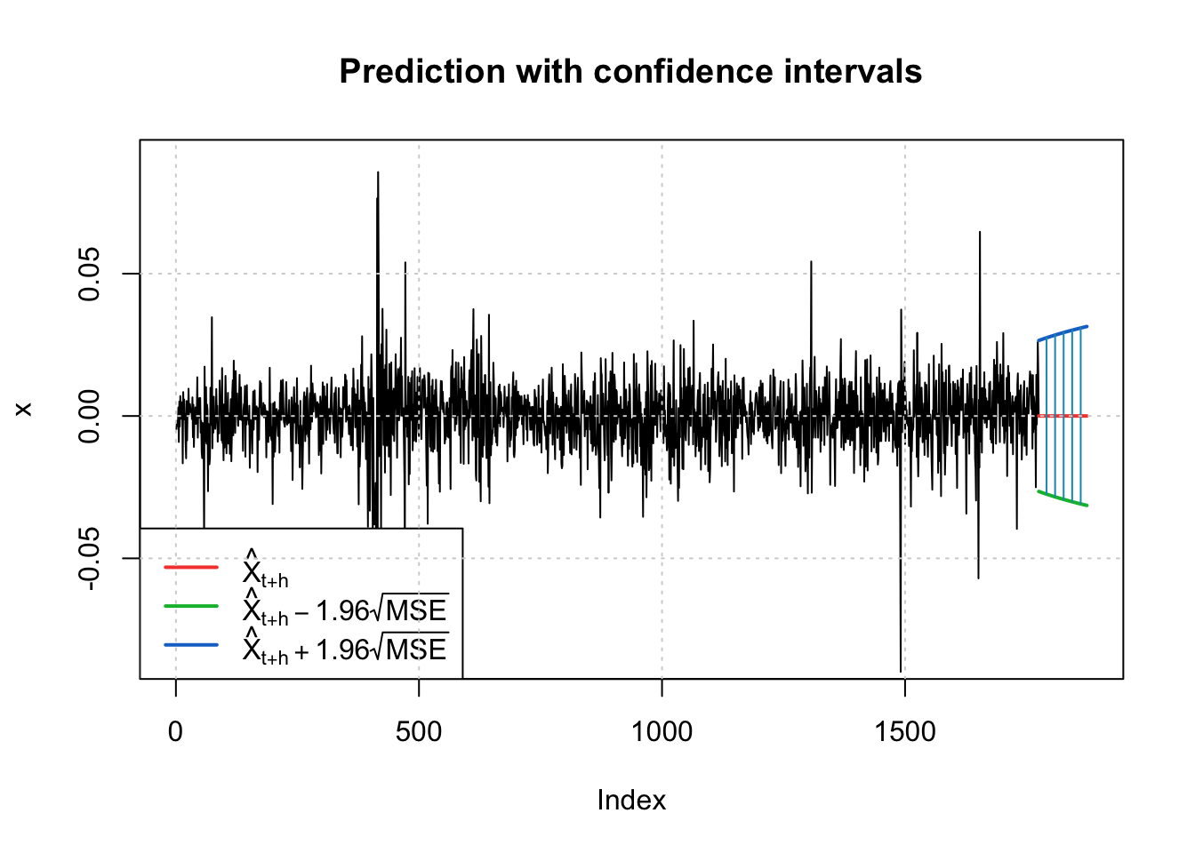
fc <-predict(final.fit1, n.ahead =100)invisible(predict(final.fit1, n.ahead =100, plot =TRUE))
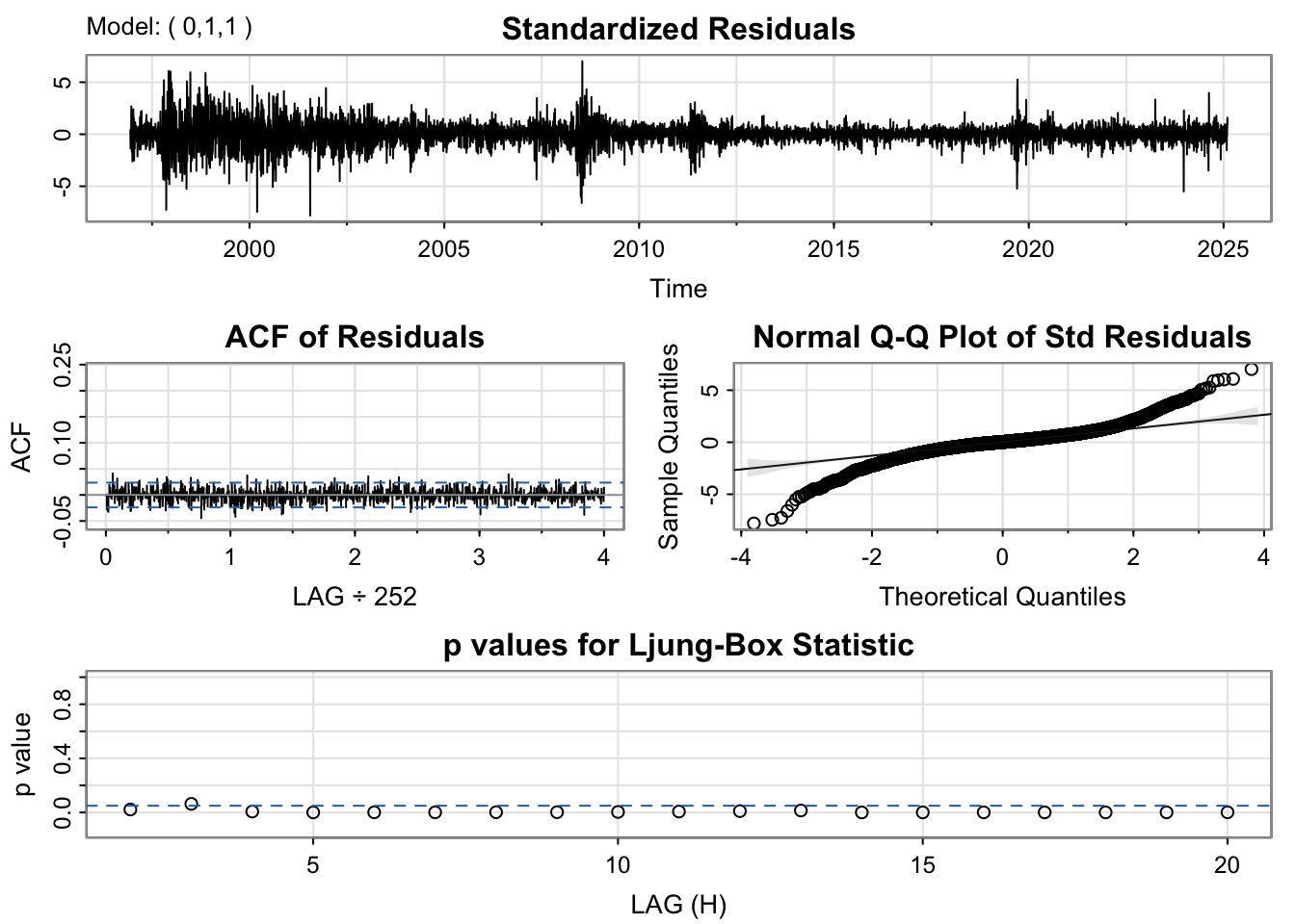
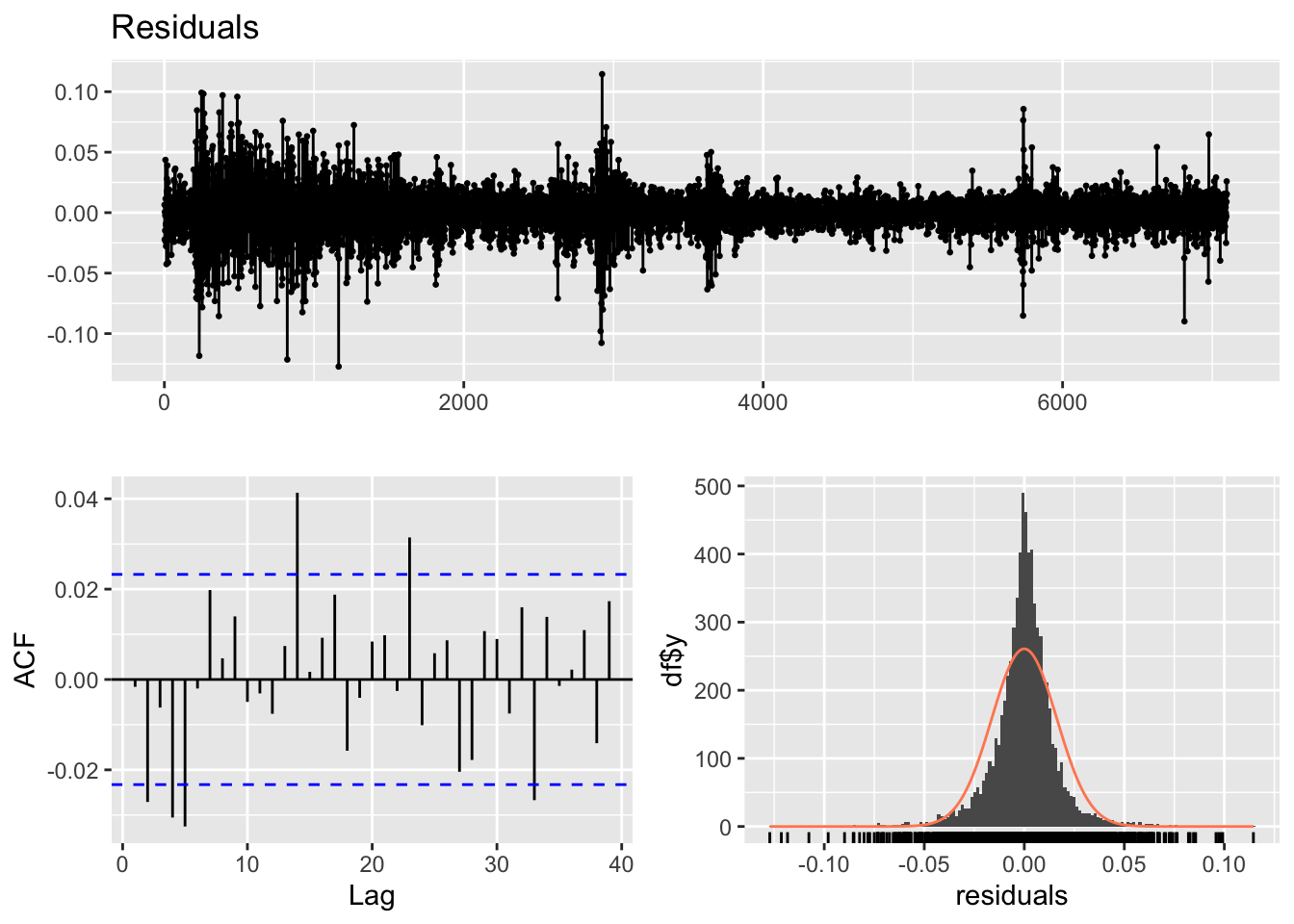
For the final model, an ARIMA(0,1,1) + GARCH(1,1) specification was used. The model diagnostics provide some insight into its performance. The residual plot shows a reasonably good pattern, with no obvious systematic structure and only a few noticeable spikes. The ACF plot of the residuals indicates that most lags fall within the significance bounds, suggesting that autocorrelation has been largely resolved.
However, the Ljung–Box test yields a very small p-value (0.007), indicating that the model fit is not fully satisfactory and that some dependence may remain in the residuals. Even so, this model is preferred because all of its coefficients are statistically significant, unlike the alternative specifications considered. Therefore, this is taken as the best model among the candidates.
In the previous modeling, the overall model fit was not satisfactory. Therefore, in this section, a different modeling approach is used: directly applying models from the ARCH/GARCH family.
kospi_acf_log <-ggAcf(kospi_return,lag.max =30)+ggtitle("ACF Plot of KOSPI Index") +theme_bw() +geom_segment(lineend ="butt", color ="orange") +geom_hline(yintercept =0, color ="orange") kospi_pacf_log <-ggPacf(kospi_return,lag.max =30)+ggtitle("PACF Plot of KOSPI Index") +theme_bw()+geom_segment(lineend ="butt", color ="skyblue") +geom_hline(yintercept =0, color ="skyblue") kospi_acf_log/kospi_pacf_log
Based on the ACF and PACF plots, the parameter search range for the manual selection process will be set from 0 to 5 for both p and q.
Code
# Initialize model storagemodels <-list()results <-data.frame(p =integer(), q =integer(), AIC =numeric())cc <-1# Grid search for GARCH(p, q), where p = ARCH order, q = GARCH orderfor (p in1:5) {for (q in1:5) { fit <-tryCatch(garch(kospi_return, order =c(q, p), trace =FALSE),error =function(e) NULL )if (!is.null(fit)) { models[[cc]] <- fit results <-rbind(results, data.frame(p = p, q = q, AIC =AIC(fit))) cc <- cc +1 } }}# Round AIC values for readabilityresults$AIC <-round(results$AIC, 3)# Identify the model with the lowest AIChighlight_row <-which.min(results$AIC)# Display formatted tableresults %>%kable(caption ="AIC Comparison for GARCH(p, q) Models",col.names =c("ARCH Order (p)", "GARCH Order (q)", "AIC"),align =c("c", "c", "c"),booktabs =TRUE ) %>%kable_styling(full_width =FALSE,position ="center",bootstrap_options =c("striped", "hover", "condensed") ) %>%row_spec(highlight_row, bold =TRUE, background ="#FFF59D")
AIC Comparison for GARCH(p, q) Models
ARCH Order (p)
GARCH Order (q)
AIC
1
1
-41720.63
1
2
-41712.15
1
3
-41700.60
1
4
-41694.91
1
5
-41657.04
2
1
-41711.77
2
2
-41710.51
2
3
-40956.99
2
4
-41716.38
2
5
-41692.39
3
1
-41601.49
3
2
-41713.82
3
3
-41673.10
3
4
-41686.95
3
5
-41676.55
4
1
-41481.96
4
2
-41771.15
4
3
-41592.23
4
4
-41687.38
4
5
-41701.31
5
1
-41494.61
5
2
-41541.75
5
3
-41679.61
5
4
-41680.56
5
5
-41694.14
Optimal model based on AIC is GARCH(4,2) model.
Code
garch_model1 <-garchFit(~garch(4,2), data = kospi_return, trace =FALSE)summary(garch_model1)
Title:
 GARCH Modelling

Call:
 garchFit(formula = ~garch(4, 2), data = kospi_return, trace = FALSE)

Mean and Variance Equation:
 data ~ garch(4, 2)
<environment: 0x10da9daa0>
 [data = kospi_return]

Conditional Distribution:
 norm

Coefficient(s):
        mu       omega      alpha1      alpha2      alpha3      alpha4
4.3079e-04  2.4548e-06  8.3322e-02  7.5768e-02  1.0000e-08  1.0000e-08
     beta1       beta2
9.7797e-02  7.3842e-01

Std. Errors:
 based on Hessian

Error Analysis:
        Estimate  Std. Error  t value Pr(>|t|)
mu     4.308e-04   1.236e-04    3.485 0.000491 ***
omega  2.455e-06   1.172e-06    2.095 0.036147 *
alpha1 8.332e-02   1.731e-02    4.813 1.49e-06 ***
alpha2 7.577e-02   6.397e-02    1.184 0.236231
alpha3 1.000e-08   3.072e-02    0.000 1.000000
alpha4 1.000e-08   1.848e-02    0.000 1.000000
beta1  9.780e-02   7.378e-01    0.133 0.894547
beta2  7.384e-01   6.668e-01    1.107 0.268102
---
Signif. codes:  0 '***' 0.001 '**' 0.01 '*' 0.05 '.' 0.1 ' ' 1

Log Likelihood:
 20871.86    normalized:  2.941355

Description:
 Thu Nov 20 15:29:27 2025 by user:


Standardised Residuals Tests:
                                  Statistic    p-Value
 Jarque-Bera Test   R    Chi^2  1164.706555 0.00000000
 Shapiro-Wilk Test  R    W               NA         NA
 Ljung-Box Test     R    Q(10)    26.923355 0.00267804
 Ljung-Box Test     R    Q(15)    30.128349 0.01146701
 Ljung-Box Test     R    Q(20)    35.002552 0.02009069
 Ljung-Box Test     R^2  Q(10)     5.823711 0.82985033
 Ljung-Box Test     R^2  Q(15)    13.124526 0.59268010
 Ljung-Box Test     R^2  Q(20)    18.795894 0.53512652
 LM Arch Test       R    TR^2      8.463032 0.74798062

Information Criterion Statistics:
      AIC       BIC       SIC      HQIC
-5.880455 -5.872713 -5.880458 -5.877789
Code
garch_model2 <-garchFit(~garch(2,1), data = kospi_return, trace =FALSE)summary(garch_model2)
Title:
 GARCH Modelling

Call:
 garchFit(formula = ~garch(2, 1), data = kospi_return, trace = FALSE)

Mean and Variance Equation:
 data ~ garch(2, 1)
<environment: 0x1333aa6f8>
 [data = kospi_return]

Conditional Distribution:
 norm

Coefficient(s):
        mu       omega      alpha1      alpha2       beta1
4.3437e-04  1.3374e-06  8.7170e-02  1.0000e-08  9.1030e-01

Std. Errors:
 based on Hessian

Error Analysis:
        Estimate  Std. Error  t value Pr(>|t|)
mu     4.344e-04   1.234e-04    3.519 0.000433 ***
omega  1.337e-06   2.546e-07    5.253 1.49e-07 ***
alpha1 8.717e-02   1.302e-02    6.696 2.15e-11 ***
alpha2 1.000e-08   1.439e-02    0.000 0.999999
beta1  9.103e-01   7.581e-03  120.083  < 2e-16 ***
---
Signif. codes:  0 '***' 0.001 '**' 0.01 '*' 0.05 '.' 0.1 ' ' 1

Log Likelihood:
 20871.64    normalized:  2.941324

Description:
 Thu Nov 20 15:29:27 2025 by user:


Standardised Residuals Tests:
                                  Statistic     p-Value
 Jarque-Bera Test   R    Chi^2  1154.123087 0.000000000
 Shapiro-Wilk Test  R    W               NA          NA
 Ljung-Box Test     R    Q(10)    26.809723 0.002791025
 Ljung-Box Test     R    Q(15)    30.007624 0.011894034
 Ljung-Box Test     R    Q(20)    34.899755 0.020644719
 Ljung-Box Test     R^2  Q(10)     5.463024 0.858183043
 Ljung-Box Test     R^2  Q(15)    12.876270 0.611854288
 Ljung-Box Test     R^2  Q(20)    18.539767 0.551896747
 LM Arch Test       R    TR^2      8.216584 0.767984231

Information Criterion Statistics:
      AIC       BIC       SIC      HQIC
-5.881239 -5.876400 -5.881240 -5.879573
Code
garch_model3 <-garchFit(~garch(1,1), data = kospi_return, trace =FALSE)summary(garch_model3)
Title:
 GARCH Modelling

Call:
 garchFit(formula = ~garch(1, 1), data = kospi_return, trace = FALSE)

Mean and Variance Equation:
 data ~ garch(1, 1)
<environment: 0x125c03078>
 [data = kospi_return]

Conditional Distribution:
 norm

Coefficient(s):
        mu       omega      alpha1       beta1
4.3479e-04  1.3385e-06  8.7224e-02  9.1024e-01

Std. Errors:
 based on Hessian

Error Analysis:
        Estimate  Std. Error  t value Pr(>|t|)
mu     4.348e-04   1.233e-04    3.525 0.000423 ***
omega  1.338e-06   2.475e-07    5.407  6.4e-08 ***
alpha1 8.722e-02   7.010e-03   12.442  < 2e-16 ***
beta1  9.102e-01   6.779e-03  134.266  < 2e-16 ***
---
Signif. codes:  0 '***' 0.001 '**' 0.01 '*' 0.05 '.' 0.1 ' ' 1

Log Likelihood:
 20871.81    normalized:  2.941349

Description:
 Thu Nov 20 15:29:27 2025 by user:


Standardised Residuals Tests:
                                  Statistic     p-Value
 Jarque-Bera Test   R    Chi^2  1154.190795 0.000000000
 Shapiro-Wilk Test  R    W               NA          NA
 Ljung-Box Test     R    Q(10)    26.785630 0.002815565
 Ljung-Box Test     R    Q(15)    29.980295 0.011992750
 Ljung-Box Test     R    Q(20)    34.874716 0.020781772
 Ljung-Box Test     R^2  Q(10)     5.464082 0.858103131
 Ljung-Box Test     R^2  Q(15)    12.886787 0.611042151
 Ljung-Box Test     R^2  Q(20)    18.551672 0.551115659
 LM Arch Test       R    TR^2      8.215222 0.768093388

Information Criterion Statistics:
      AIC       BIC       SIC      HQIC
-5.881571 -5.877700 -5.881572 -5.880238
When testing the model with the lowest AIC, the overall fit was strong; however, not all coefficients were statistically significant, with some showing large p-values. Therefore, two additional models were considered: one with an AIC value close to the minimum and another specified as GARCH(1,1).Comparing the three models, all coefficients in the GARCH(1,1) model were significant, so this model is selected as the final choice.
Code
garch.fit2 <-garch(kospi_return, order =c(1,1), trace =FALSE) summary(garch.fit2)
    Ljung-Box test

data:  Residuals
Q* = 533.52, df = 504, p-value = 0.1754

Model df: 0.   Total lags used: 504
From model diagnostics, this model shows similar result for ACF and residual plot compare to other model approach. However, for Ljung-Box test, it has much better p-value, indicating that this model has better model fit compare to other method.
p_us <-plot_ly(kr, x =~Date, y =~krw, type ="scatter", mode ="lines",name ="USD per KRW") %>%layout(title ="USD per KRW",xaxis =list(title ="Date"),yaxis =list(title ="USD per KRW"))p_us
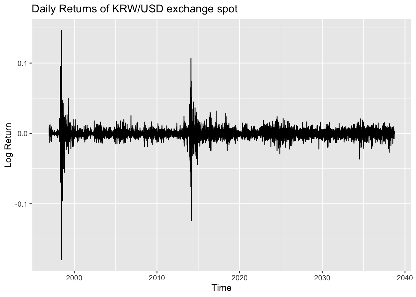
As discussed in the univariate and multivariate time series model sections, for exchange rate data,log transformation data didn’t perform well, so original data was applied. The first plot is a time series plot of the KRW/USD exchange spot. Plot shows when there is an economic crisis(ex.2009 financial crisis), KRW against USD increases significantly.
The second plot shows the returns of theKRW/USD exchange spot. In this plot, volatility clustering is clearly observed: for most periods, the values are centered near zero, but in certain periods the series exhibits high volatility before returning to calmer behavior. This suggests that the data are potentially appropriate for modeling with the ARCH/GARCH family of models.
library(patchwork)kr_acf <-ggAcf(kr_return,lag.max =30)+ggtitle("ACF Plot of KRW/USD exchange spot") +theme_bw() +geom_segment(lineend ="butt", color ="orange") +geom_hline(yintercept =0, color ="orange") kr_pacf <-ggPacf(kr_return,lag.max =30)+ggtitle("PACF Plot of KRW/USD exchange spot") +theme_bw()+geom_segment(lineend ="butt", color ="skyblue") +geom_hline(yintercept =0, color ="skyblue") kr_acf/kr_pacf
From the plots, KOSPI Index data performs well in terms of autocorrelation by applying log transformation, However there are still some lag points showing autocorrelation.
p-vlaue is smaller than 0.05(default criterion), indicating rejecting null hypothesis, concluding strong evidence for the presence of ARCH(1) effects in the data.
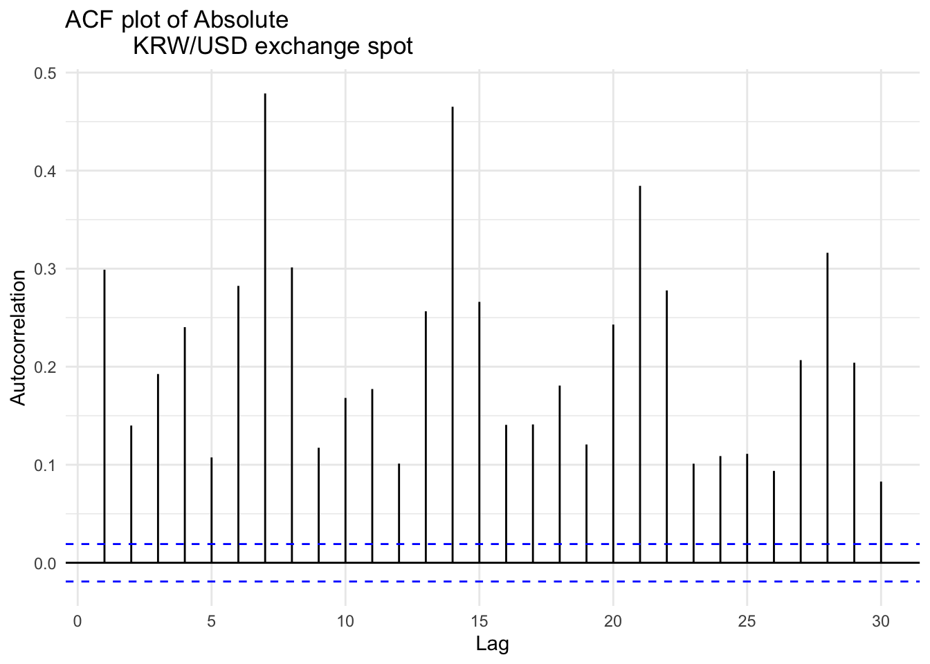
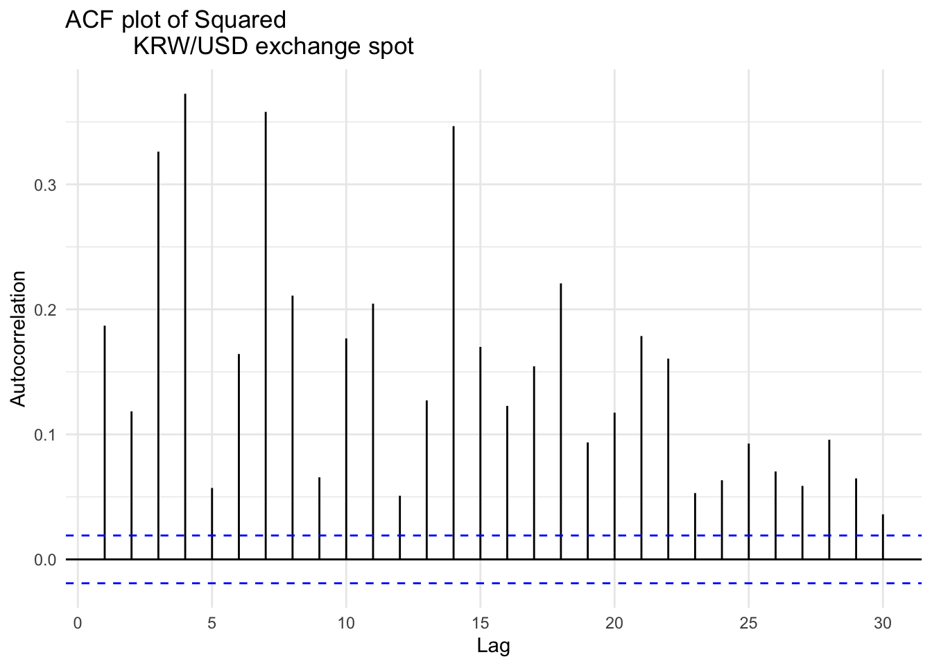
Two plots for applying absolute value and squaring to KRW/USD exchange spot shows significant autocorrelation throughout multiple lags, compare to log return. This implies that the returns are not independently and identically distributed, and gives evidence for need to apply conditional variance models such as ARCH or GARCH to capture the underlying time-varying volatility structure.
library(patchwork)kr_acf <-ggAcf(kr_ts,lag.max =30)+ggtitle("ACF Plot of KRW/USD exchange spot ") +theme_bw() +geom_segment(lineend ="butt", color ="orange") +geom_hline(yintercept =0, color ="orange") kr_pacf <-ggPacf(kr_ts,lag.max =30)+ggtitle("PACF Plot of KRW/USD exchange spot") +theme_bw()+geom_segment(lineend ="butt", color ="skyblue") +geom_hline(yintercept =0, color ="skyblue") kr_acf/kr_pacf
Code
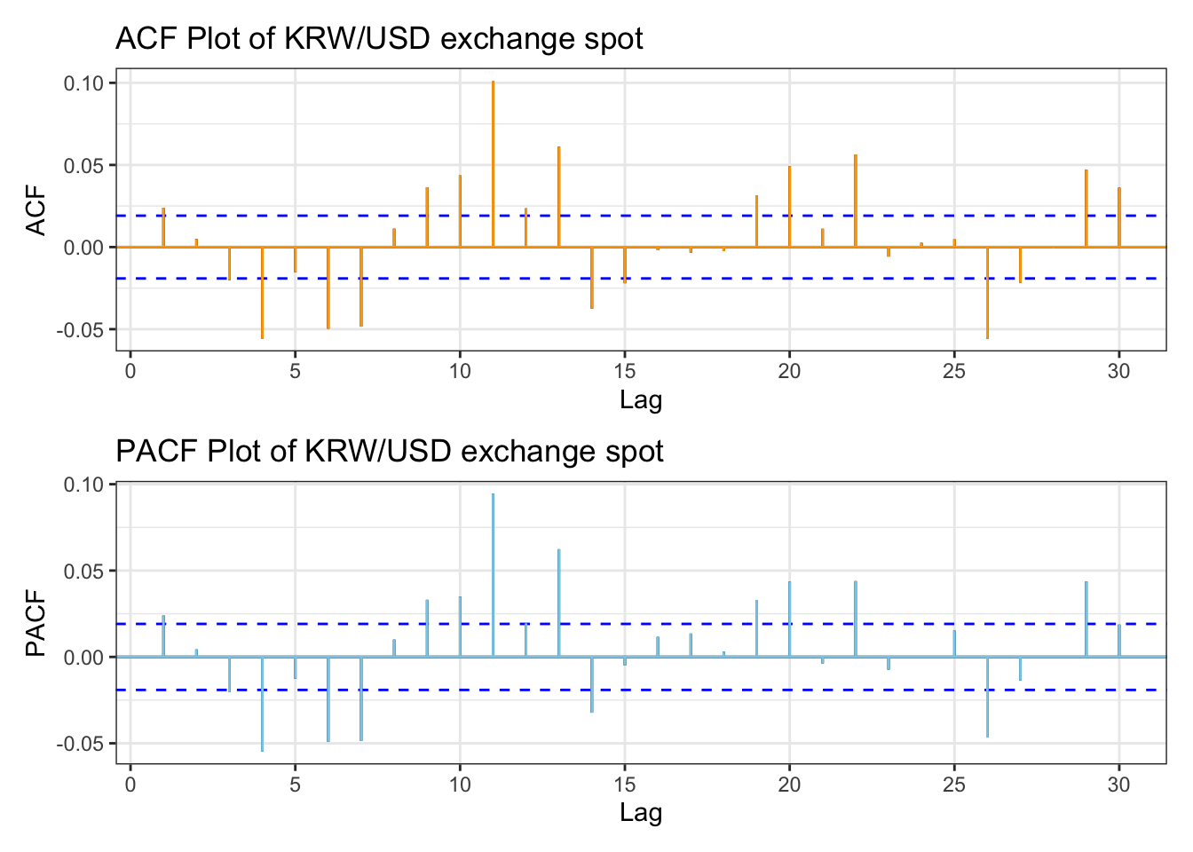
kr_acf_log <-ggAcf(kr_return,lag.max =30)+ggtitle("ACF Plot of KRW/USD exchange spot") +theme_bw() +geom_segment(lineend ="butt", color ="orange") +geom_hline(yintercept =0, color ="orange") kr_pacf_log <-ggPacf(kr_return,lag.max =30)+ggtitle("PACF Plot of KRW/USD exchange spot") +theme_bw()+geom_segment(lineend ="butt", color ="skyblue") +geom_hline(yintercept =0, color ="skyblue") kr_acf_log/kr_pacf_log
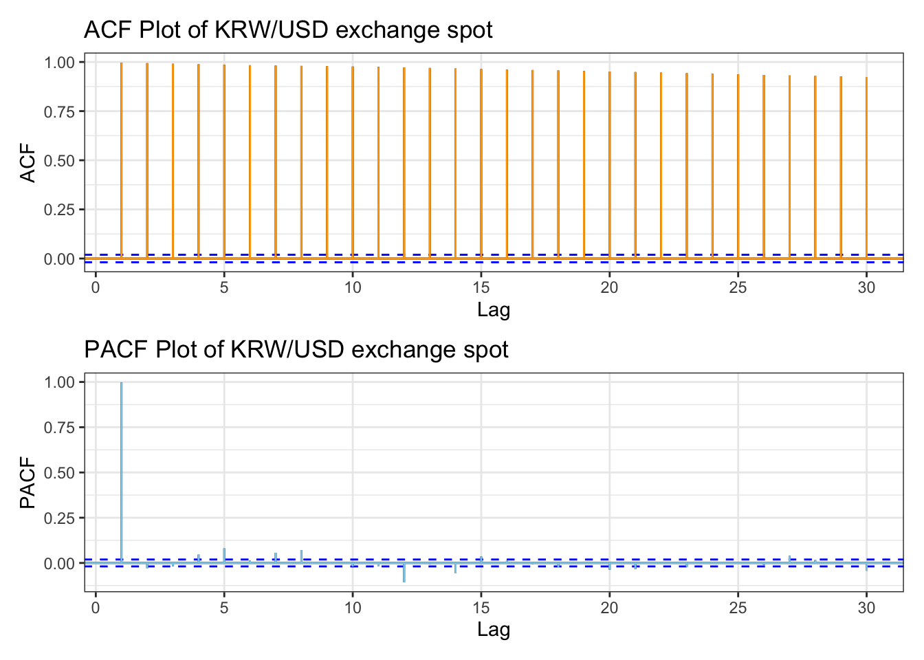
ACF plot shows significant autocorrelation across lags. Also in the PACF plot, it has significant autocorrelation, then drops significantly, indicating almost no autocorrelation after lag1.these plots indicate the presence of dependencies between past and current price movements, series is stationary.
ACF and PACF plot for KRW/USD exchange spot return shows that most of the lags are within threshold, however there are lags that spike, for example like lag4. For manual search, a search range from 0 to 4 seems appropriate.
And both plots have similar patterns, indicating that conditional heteroskedasticity is present. So applying the ARCH/GARCH family model is appropriate.
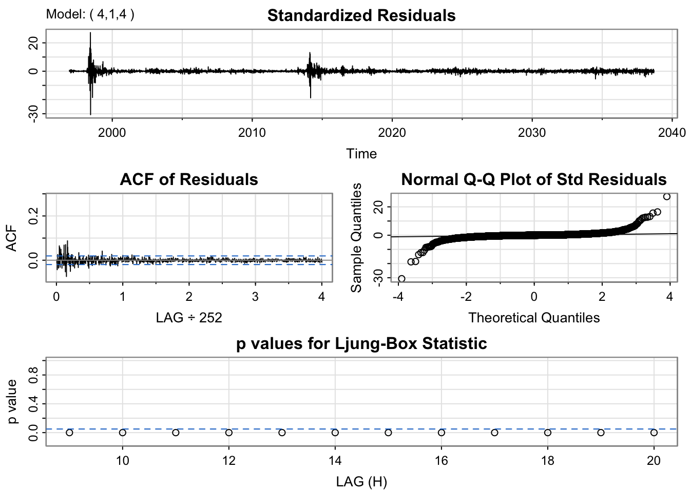
From model diagnostic for three potential models, diagnostics are not satisfactory, to evaluate which model to choose, model AIC,BIC and coefficient’s significance. In this sense, i would use ARIMA(4,1,4) model since it has lowest BIC value. Also auto.arima() suggested ARIMA(0,1,0)(0,0,1)[252], however as seen in EDA and univariate section, using ARIMA(4,1,4) is more appropriate.
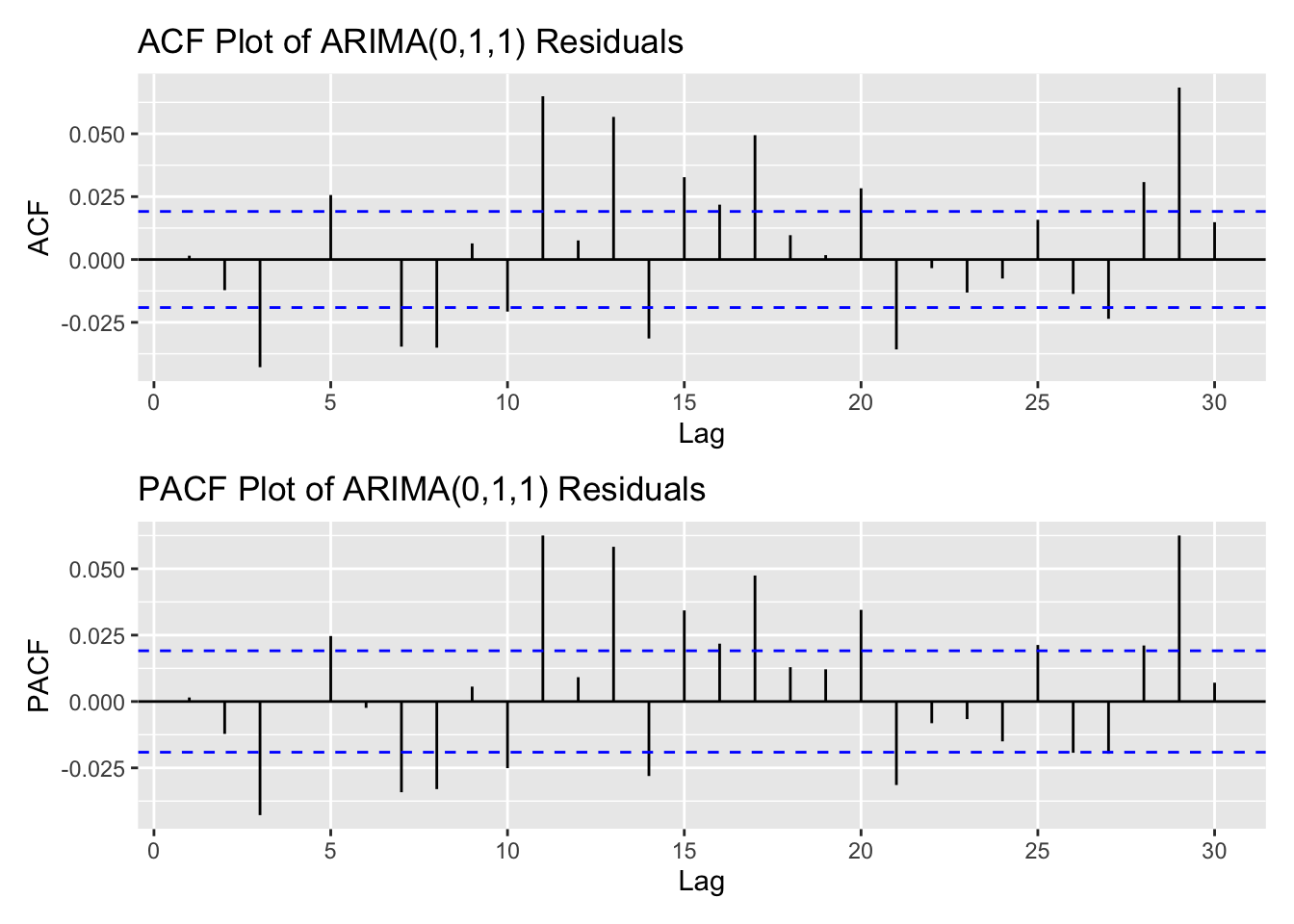
arima_fit2 <-Arima(kr_ts, order =c(4,1,4), include.drift =TRUE)res_arima2<-residuals(arima_fit2)kr_res_acf <-ggAcf(res_arima2,lag.max =30)+ggtitle("ACF Plot of ARIMA(0,1,1) Residuals") kr_res_pacf <-ggPacf(res_arima2,lag.max =30)+ggtitle("PACF Plot of ARIMA(0,1,1) Residuals") kr_res_acf/kr_res_pacf
Code
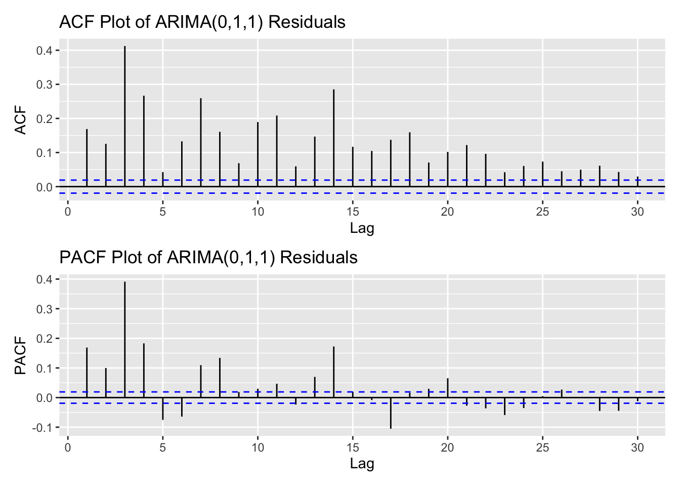
kr_res_acf <-ggAcf(res_arima2^2,lag.max =30)+ggtitle("ACF Plot of ARIMA(0,1,1) Residuals") kr_res_pacf <-ggPacf(res_arima2^2,lag.max =30)+ggtitle("PACF Plot of ARIMA(0,1,1) Residuals") kr_res_acf/kr_res_pacf
From the ACF and PACF plots of the residuals and squared residuals for the ARIMA(4,1,4) model, the ACF of the squared residuals shows noticeable spikes up to lag 4, followed by a gradual decline. This suggests the presence of an ARCH effect, indicating time-varying volatility in the data. Based on these plots, an appropriate range for manual model search is p,q both in 0:4 range.
Code
library(tseries)library(knitr)library(kableExtra)# Initialize list to store models and track p, qmodels <-list()pq_combinations <-data.frame(p =integer(), q =integer(), AIC =numeric())cc <-1for (p in0:4) {for (q in0:4) { fit <-tryCatch(garch(res_arima2, order =c(q, p), trace =FALSE),error =function(e) NULL )if (!is.null(fit)) { models[[cc]] <- fit pq_combinations <-rbind( pq_combinations,data.frame(p = p, q = q, AIC =AIC(fit)) ) cc <- cc +1 } }}# Round AIC for presentationpq_combinations$AIC <-round(pq_combinations$AIC, 3)# Identify row with minimum AIChighlight_row <-which.min(pq_combinations$AIC)# Create formatted tablepq_combinations %>%kable(caption ="AIC Comparison for GARCH(p, q) Models",col.names =c("ARCH Order (p)", "GARCH Order (q)", "AIC"),align =c("c", "c", "c"),booktabs =TRUE ) %>%kable_styling(full_width =FALSE,position ="center",bootstrap_options =c("striped", "hover", "condensed") ) %>%row_spec(highlight_row, bold =TRUE, background ="#FFF59D")
AIC Comparison for GARCH(p, q) Models
ARCH Order (p)
GARCH Order (q)
AIC
0
1
77039.26
0
2
77034.41
0
3
77030.07
0
4
77025.75
1
0
70886.82
1
1
64300.52
1
2
72349.90
1
3
72043.93
1
4
71748.54
2
0
69232.85
2
1
64279.30
2
2
71642.42
2
3
71336.80
2
4
70970.01
3
0
67892.56
3
1
71271.64
3
2
70976.80
3
3
70627.55
3
4
70299.92
4
0
66876.25
4
1
70645.10
4
2
70323.57
4
3
69988.46
4
4
69621.45
From manual search, GARCH(2,1) model is better has lowest AIC
Code
cat("\nSummary for GARCH(2,1):\n")
Summary for GARCH(2,1):
Code
garch_model <-garchFit(~garch(2, 1), data = res_arima2, trace =FALSE)summary(garch_model)
Title:
 GARCH Modelling

Call:
 garchFit(formula = ~garch(2, 1), data = res_arima2, trace = FALSE)

Mean and Variance Equation:
 data ~ garch(2, 1)
<environment: 0x116756070>
 [data = res_arima2]

Conditional Distribution:
 norm

Coefficient(s):
         mu        omega       alpha1       alpha2        beta1
-0.00360202   0.11451836   0.06124867   0.00000001   0.94049761

Std. Errors:
 based on Hessian

Error Analysis:
         Estimate  Std. Error  t value Pr(>|t|)
mu     -3.602e-03   3.977e-02   -0.091    0.928
omega   1.145e-01   6.631e-03   17.271   <2e-16 ***
alpha1  6.125e-02   7.269e-03    8.426   <2e-16 ***
alpha2  1.000e-08   7.986e-03    0.000    1.000
beta1   9.405e-01   2.357e-03  398.977   <2e-16 ***
---
Signif. codes:  0 '***' 0.001 '**' 0.01 '*' 0.05 '.' 0.1 ' ' 1

Log Likelihood:
 -32172.01    normalized:  -3.057014

Description:
 Thu Nov 20 15:31:15 2025 by user:


Standardised Residuals Tests:
                                  Statistic      p-Value
 Jarque-Bera Test   R    Chi^2  16959.12128 0.000000e+00
 Shapiro-Wilk Test  R    W               NA           NA
 Ljung-Box Test     R    Q(10)    130.21986 0.000000e+00
 Ljung-Box Test     R    Q(15)    138.42008 0.000000e+00
 Ljung-Box Test     R    Q(20)    151.96975 0.000000e+00
 Ljung-Box Test     R^2  Q(10)     53.38745 6.308545e-08
 Ljung-Box Test     R^2  Q(15)     85.45499 6.931011e-12
 Ljung-Box Test     R^2  Q(20)    101.05036 8.166801e-13
 LM Arch Test       R    TR^2      59.11074 3.276980e-08

Information Criterion Statistics:
     AIC      BIC      SIC     HQIC
6.114977 6.118427 6.114977 6.116142
Code
cat("\nSummary for GARCH(1,1):\n")
Summary for GARCH(1,1):
Code
garch_model <-garchFit(~garch(1,1), data = res_arima2, trace =FALSE)summary(garch_model)
Title:
 GARCH Modelling

Call:
 garchFit(formula = ~garch(1, 1), data = res_arima2, trace = FALSE)

Mean and Variance Equation:
 data ~ garch(1, 1)
<environment: 0x143edfb50>
 [data = res_arima2]

Conditional Distribution:
 norm

Coefficient(s):
       mu      omega     alpha1      beta1
-0.003602   0.114441   0.061231   0.940516

Std. Errors:
 based on Hessian

Error Analysis:
        Estimate  Std. Error  t value Pr(>|t|)
mu     -0.003602    0.039752   -0.091    0.928
omega   0.114441    0.006616   17.298   <2e-16 ***
alpha1  0.061231    0.002842   21.543   <2e-16 ***
beta1   0.940516    0.002166  434.227   <2e-16 ***
---
Signif. codes:  0 '***' 0.001 '**' 0.01 '*' 0.05 '.' 0.1 ' ' 1

Log Likelihood:
 -32171.35    normalized:  -3.056951

Description:
 Thu Nov 20 15:31:15 2025 by user:


Standardised Residuals Tests:
                                  Statistic      p-Value
 Jarque-Bera Test   R    Chi^2  16956.04373 0.000000e+00
 Shapiro-Wilk Test  R    W               NA           NA
 Ljung-Box Test     R    Q(10)    130.23088 0.000000e+00
 Ljung-Box Test     R    Q(15)    138.41555 0.000000e+00
 Ljung-Box Test     R    Q(20)    151.97084 0.000000e+00
 Ljung-Box Test     R^2  Q(10)     53.39726 6.282115e-08
 Ljung-Box Test     R^2  Q(15)     85.44565 6.958656e-12
 Ljung-Box Test     R^2  Q(20)    101.05454 8.152368e-13
 LM Arch Test       R    TR^2      59.12034 3.263836e-08

Information Criterion Statistics:
     AIC      BIC      SIC     HQIC
6.114662 6.117422 6.114662 6.115594
By manual search to find optimal p,q value, GARCH(2,1) had lowest AIC. However when fitting a model with this parameter, alpha2 are not significant with large p value, trying other close by AIC values could be appropriate. After testing more model, all the coefficient for GARCH(1,1) model are significant and very close AIC value to lowest value, So further modeling GARCH(1,1) will be used.
Code
arima_fit2 <-Arima(kr_ts, order =c(4,1,4), include.drift =TRUE)arima_res2<-residuals(arima_fit2)final.fit20<-garchFit(~garch(1, 1), data = arima_res2, trace =FALSE)summary(final.fit20)
Title:
 GARCH Modelling

Call:
 garchFit(formula = ~garch(1, 1), data = arima_res2, trace = FALSE)

Mean and Variance Equation:
 data ~ garch(1, 1)
<environment: 0x10f56b7b0>
 [data = arima_res2]

Conditional Distribution:
 norm

Coefficient(s):
       mu      omega     alpha1      beta1
-0.003602   0.114441   0.061231   0.940516

Std. Errors:
 based on Hessian

Error Analysis:
        Estimate  Std. Error  t value Pr(>|t|)
mu     -0.003602    0.039752   -0.091    0.928
omega   0.114441    0.006616   17.298   <2e-16 ***
alpha1  0.061231    0.002842   21.543   <2e-16 ***
beta1   0.940516    0.002166  434.227   <2e-16 ***
---
Signif. codes:  0 '***' 0.001 '**' 0.01 '*' 0.05 '.' 0.1 ' ' 1

Log Likelihood:
 -32171.35    normalized:  -3.056951

Description:
 Thu Nov 20 15:31:16 2025 by user:


Standardised Residuals Tests:
                                  Statistic      p-Value
 Jarque-Bera Test   R    Chi^2  16956.04373 0.000000e+00
 Shapiro-Wilk Test  R    W               NA           NA
 Ljung-Box Test     R    Q(10)    130.23088 0.000000e+00
 Ljung-Box Test     R    Q(15)    138.41555 0.000000e+00
 Ljung-Box Test     R    Q(20)    151.97084 0.000000e+00
 Ljung-Box Test     R^2  Q(10)     53.39726 6.282115e-08
 Ljung-Box Test     R^2  Q(15)     85.44565 6.958656e-12
 Ljung-Box Test     R^2  Q(20)    101.05454 8.152368e-13
 LM Arch Test       R    TR^2      59.12034 3.263836e-08

Information Criterion Statistics:
     AIC      BIC      SIC     HQIC
6.114662 6.117422 6.114662 6.115594
    Ljung-Box test

data:  Residuals
Q* = 58.374, df = 10, p-value = 7.351e-09

Model df: 0.   Total lags used: 10
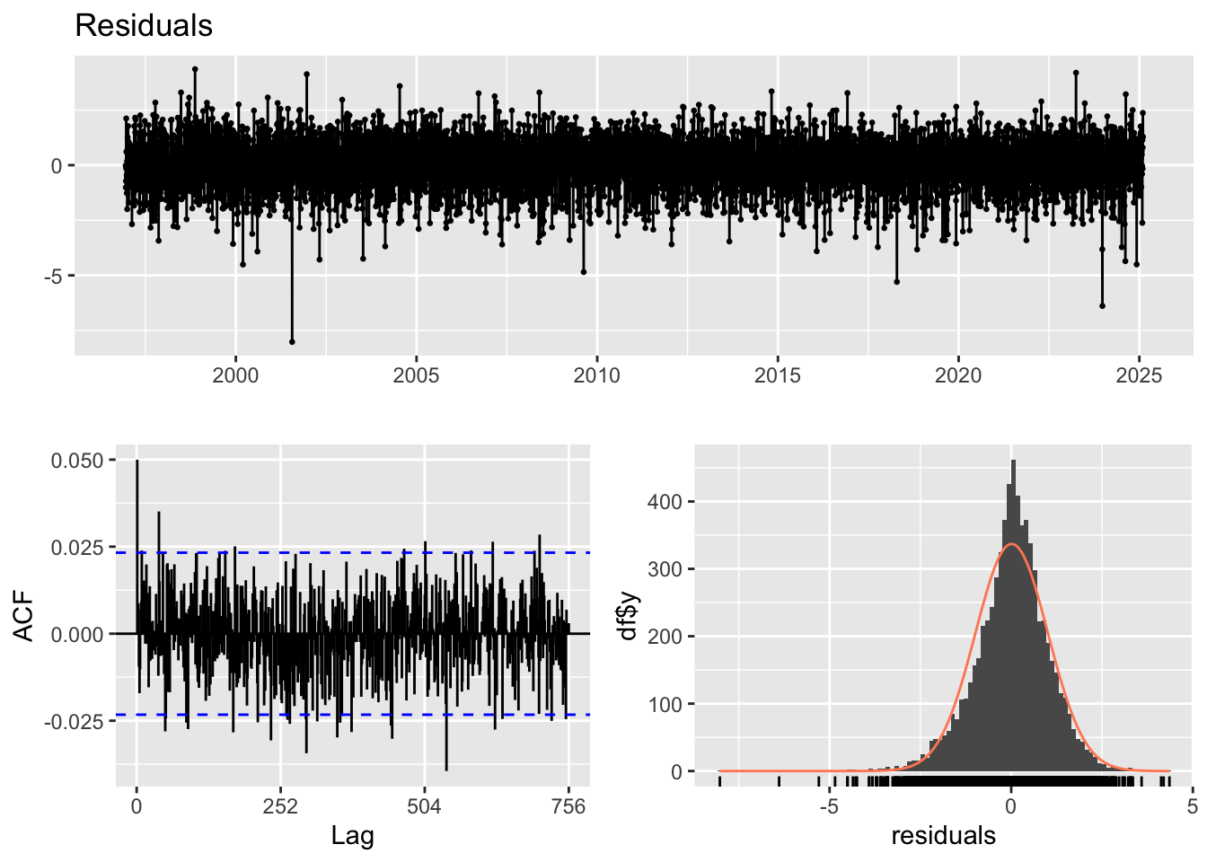
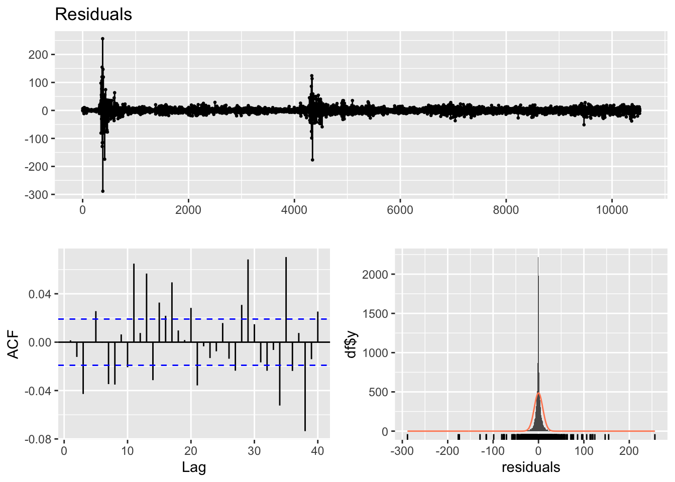
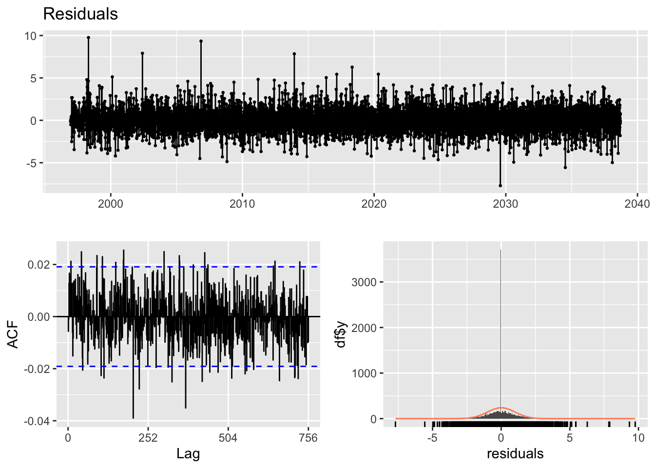
For final model, ARIMA(4,1,4)+GARCH(1,1) model was used. Model diagnostic give some intuition for this model. First residual plot shows it is good patterns, similar patterns with spikes. ACF plot also shows most lags fall into threshold, autocorrelation is resolved. however , for Ljung-Box test, it has very small p-value, indicating model fit is not satisfactory. However this model give all the coefficients as significant compare to other model choice, so this is the best model.
Code
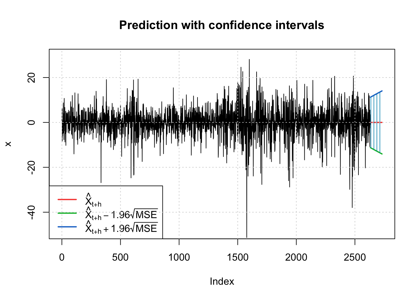
fc <-predict(final.fit20, n.ahead =100)invisible(predict(final.fit20, n.ahead =100, plot =TRUE))
In the previous modeling, the overall model fit was not satisfactory. Therefore, in this section, a different modeling approach is used: directly applying models from the ARCH/GARCH family.
kr_acf_log <-ggAcf(kr_return,lag.max =30)+ggtitle("ACF Plot of KRW/USD exchange spot") +theme_bw() +geom_segment(lineend ="butt", color ="orange") +geom_hline(yintercept =0, color ="orange") kr_pacf_log <-ggPacf(kr_return,lag.max =30)+ggtitle("PACF Plot of KRW/USD exchange spot") +theme_bw()+geom_segment(lineend ="butt", color ="skyblue") +geom_hline(yintercept =0, color ="skyblue") kr_acf_log/kr_pacf_log
Based on the ACF and PACF plots, the parameter search range for the manual selection process will be set from 0 to 5 for both p and q.
Code
# Initialize model storagemodels <-list()results <-data.frame(p =integer(), q =integer(), AIC =numeric())cc <-1# Grid search for GARCH(p, q), where p = ARCH order, q = GARCH orderfor (p in1:5) {for (q in1:5) { fit <-tryCatch(garch(kr_return, order =c(q, p), trace =FALSE),error =function(e) NULL )if (!is.null(fit)) { models[[cc]] <- fit results <-rbind(results, data.frame(p = p, q = q, AIC =AIC(fit))) cc <- cc +1 } }}# Round AIC values for readabilityresults$AIC <-round(results$AIC, 3)# Identify the model with the lowest AIChighlight_row <-which.min(results$AIC)# Display formatted tableresults %>%kable(caption ="AIC Comparison for GARCH(p, q) Models",col.names =c("ARCH Order (p)", "GARCH Order (q)", "AIC"),align =c("c", "c", "c"),booktabs =TRUE ) %>%kable_styling(full_width =FALSE,position ="center",bootstrap_options =c("striped", "hover", "condensed") ) %>%row_spec(highlight_row, bold =TRUE, background ="#FFF59D")
AIC Comparison for GARCH(p, q) Models
ARCH Order (p)
GARCH Order (q)
AIC
1
1
-84358.85
1
2
-84401.44
1
3
-84442.49
1
4
-84348.65
1
5
-84292.71
2
1
-83678.21
2
2
-83696.71
2
3
-84394.17
2
4
-84379.66
2
5
-84427.60
3
1
-83394.70
3
2
-83879.07
3
3
-84180.02
3
4
-84387.80
3
5
-84269.48
4
1
-82948.93
4
2
-83631.44
4
3
-84134.03
4
4
-84261.40
4
5
-84342.08
5
1
-82541.62
5
2
-84151.89
5
3
-84297.51
5
4
-84156.74
5
5
-84274.88
Code
garch_model2 <-garchFit(~garch(1,3), data = kr_return, trace =FALSE)summary(garch_model2)
Title:
 GARCH Modelling

Call:
 garchFit(formula = ~garch(1, 3), data = kr_return, trace = FALSE)

Mean and Variance Equation:
 data ~ garch(1, 3)
<environment: 0x12583e050>
 [data = kr_return]

Conditional Distribution:
 norm

Coefficient(s):
         mu        omega       alpha1        beta1        beta2        beta3
-3.4304e-05   3.2428e-07   1.2827e-01   2.6771e-02   3.9511e-01   4.4352e-01

Std. Errors:
 based on Hessian

Error Analysis:
         Estimate  Std. Error  t value Pr(>|t|)
mu     -3.430e-05   3.581e-05   -0.958    0.338
omega   3.243e-07   4.161e-08    7.793 6.44e-15 ***
alpha1  1.283e-01   6.864e-03   18.687  < 2e-16 ***
beta1   2.677e-02   3.703e-02    0.723    0.470
beta2   3.951e-01   4.189e-02    9.431  < 2e-16 ***
beta3   4.435e-01   3.712e-02   11.947  < 2e-16 ***
---
Signif. codes:  0 '***' 0.001 '**' 0.01 '*' 0.05 '.' 0.1 ' ' 1

Log Likelihood:
 42238.13    normalized:  4.013887

Description:
 Thu Nov 20 15:31:17 2025 by user:


Standardised Residuals Tests:
                                  Statistic      p-Value
 Jarque-Bera Test   R    Chi^2  17181.83321 0.000000e+00
 Shapiro-Wilk Test  R    W               NA           NA
 Ljung-Box Test     R    Q(10)     13.39087 2.026311e-01
 Ljung-Box Test     R    Q(15)     19.00019 2.137254e-01
 Ljung-Box Test     R    Q(20)     24.62524 2.161461e-01
 Ljung-Box Test     R^2  Q(10)     42.25240 6.761575e-06
 Ljung-Box Test     R^2  Q(15)     80.78765 5.011846e-11
 Ljung-Box Test     R^2  Q(20)     96.78413 4.718337e-12
 LM Arch Test       R    TR^2      49.25894 1.884473e-06

Information Criterion Statistics:
      AIC       BIC       SIC      HQIC
-8.026633 -8.022493 -8.026634 -8.025235
Code
garch_model3 <-garchFit(~garch(1,1), data = kr_return, trace =FALSE)summary(garch_model3)
Title:
 GARCH Modelling

Call:
 garchFit(formula = ~garch(1, 1), data = kr_return, trace = FALSE)

Mean and Variance Equation:
 data ~ garch(1, 1)
<environment: 0x141592cc0>
 [data = kr_return]

Conditional Distribution:
 norm

Coefficient(s):
         mu        omega       alpha1        beta1
-3.1171e-05   1.3193e-07   5.4492e-02   9.4310e-01

Std. Errors:
 based on Hessian

Error Analysis:
         Estimate  Std. Error  t value Pr(>|t|)
mu     -3.117e-05   3.612e-05   -0.863    0.388
omega   1.319e-07   1.499e-08    8.803   <2e-16 ***
alpha1  5.449e-02   2.668e-03   20.425   <2e-16 ***
beta1   9.431e-01   2.356e-03  400.327   <2e-16 ***
---
Signif. codes:  0 '***' 0.001 '**' 0.01 '*' 0.05 '.' 0.1 ' ' 1

Log Likelihood:
 42186.13    normalized:  4.008945

Description:
 Thu Nov 20 15:31:17 2025 by user:


Standardised Residuals Tests:
                                  Statistic      p-Value
 Jarque-Bera Test   R    Chi^2  15425.25000 0.000000e+00
 Shapiro-Wilk Test  R    W               NA           NA
 Ljung-Box Test     R    Q(10)     13.91883 1.767264e-01
 Ljung-Box Test     R    Q(15)     19.60159 1.877548e-01
 Ljung-Box Test     R    Q(20)     24.83351 2.078750e-01
 Ljung-Box Test     R^2  Q(10)     59.56276 4.384453e-09
 Ljung-Box Test     R^2  Q(15)     98.10012 2.986500e-14
 Ljung-Box Test     R^2  Q(20)    116.40080 1.332268e-15
 LM Arch Test       R    TR^2      64.93725 2.800070e-09

Information Criterion Statistics:
      AIC       BIC       SIC      HQIC
-8.017129 -8.014369 -8.017130 -8.016197
The optimal model based on AIC is the GARCH(1,3) model. When testing the model with the lowest AIC, the overall fit was strong; however, not all coefficients were statistically significant, with some showing large p-values. Therefore, additional model were considered: GARCH(1,1).Comparing the two models, all coefficients in the GARCH(1,1) model were significant, so this model is selected as the final choice.
Code
garch.fit2 <-garch(kr_return, order =c(1,1), trace =FALSE) summary(garch.fit2)
    Ljung-Box test

data:  Residuals
Q* = 563.01, df = 504, p-value = 0.03503

Model df: 0.   Total lags used: 504
From model diagnostics, this model shows similar result for ACF and residual plot compare to other model approach. However, for Ljung-Box test, it has much better p-value, indicating that this model has better model fit compare to other method.