The previous section examined financial time series models for the South Korean won spot exchange rate against the USD. Building on that, this section shifts the focus to deep learning methods and analyzes two key macro-financial channels: the government bond yield spread between South Korea and the United States, and South Korea’s exports to the United States. Together, these variables capture how Korea’s economy co-moves with U.S. financial conditions and external demand, providing a richer perspective than exchange rates alone.
The first part of the analysis applies recurrent neural networks to the 3-year and 10-year U.S.–Korea government bond yield spreads. These spreads summarize differences in monetary policy stance, growth expectations, and risk sentiment across the two countries, and thus serve as a compact indicator of Korea’s financial conditions relative to the U.S.
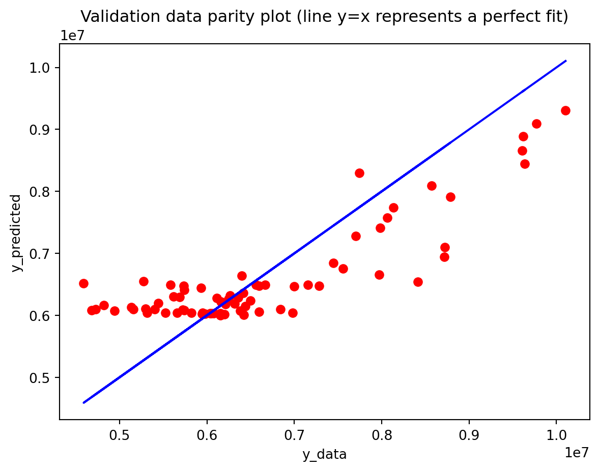
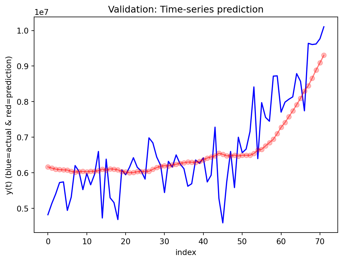
The second part extends the framework to a multivariate setting, modeling South Korea’s exports to the U.S. (in thousand dollars) jointly with several key drivers: U.S. industrial production, U.S. equity market risk (VIX), and the KRW/USD exchange rate. This multivariate specification treats exports and their main external determinants as an interconnected system rather than as separate series, allowing the model to reflect how shifts in U.S. demand, global risk sentiment, and exchange rates translate into movements in South Korean exports to the U.S.
==================================================
Training RNN...
Parameters: 32,129
==================================================
✓ Training completed in 346.32s
  Epochs trained: 111
  Best epoch: 86
  Final train loss: 0.000872
  Final val loss: 0.000819
==================================================
Training LSTM...
Parameters: 128,417
==================================================
✓ Training completed in 369.71s
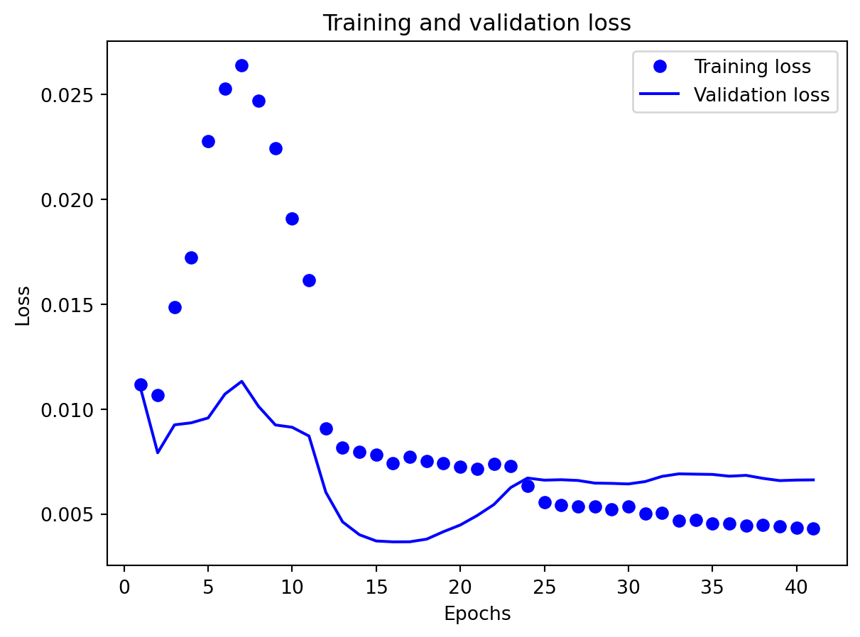
Epochs trained: 41
Best epoch: 16
Final train loss: 0.004304
Final val loss: 0.006624
==================================================
Training GRU...
Parameters: 96,993
==================================================
✓ Training completed in 501.19s
  Epochs trained: 60
  Best epoch: 35
  Final train loss: 0.006739
  Final val loss: 0.002946
==================================================
Training RNN...
Parameters: 32,129
==================================================
✓ Training completed in 315.03s
  Epochs trained: 104
  Best epoch: 79
  Final train loss: 0.000791
  Final val loss: 0.000528
==================================================
Training LSTM...
Parameters: 128,417
==================================================
✓ Training completed in 1222.75s
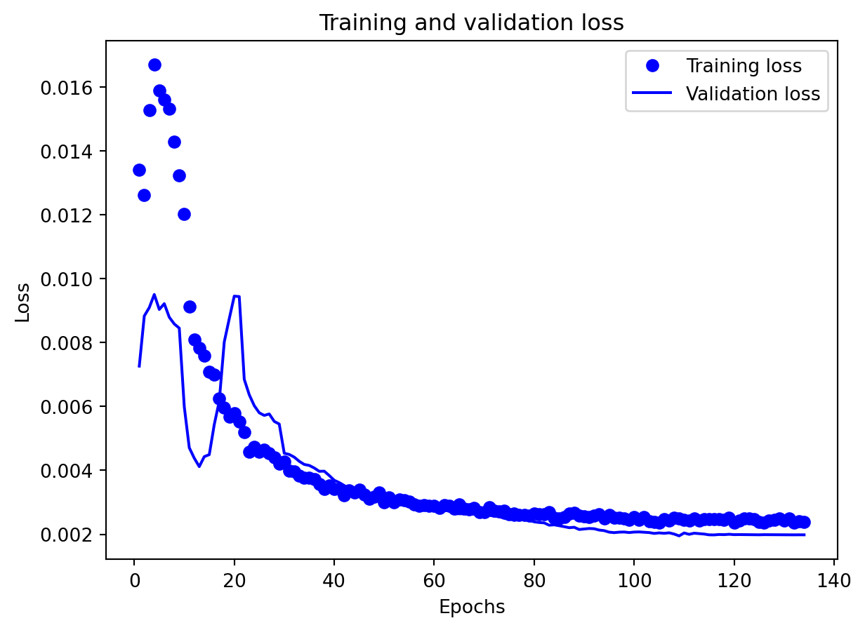
Epochs trained: 134
Best epoch: 109
Final train loss: 0.002378
Final val loss: 0.001982
==================================================
Training GRU...
Parameters: 96,993
==================================================
✓ Training completed in 1028.63s
  Epochs trained: 130
  Best epoch: 105
  Final train loss: 0.001668
  Final val loss: 0.001350
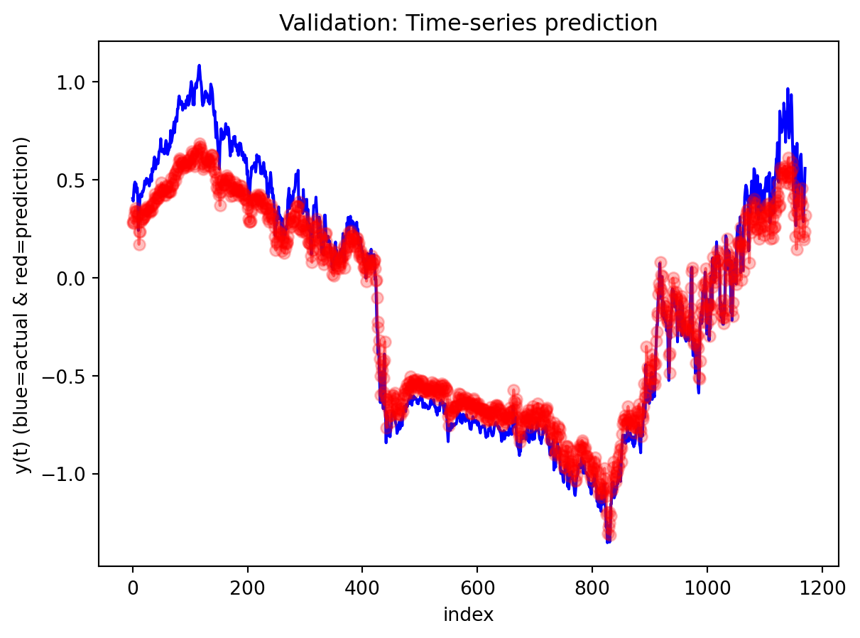
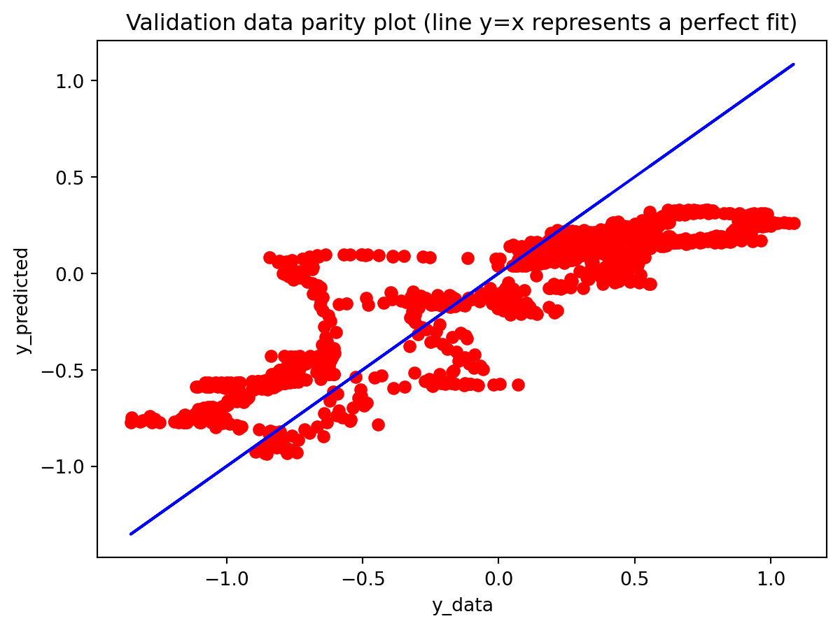
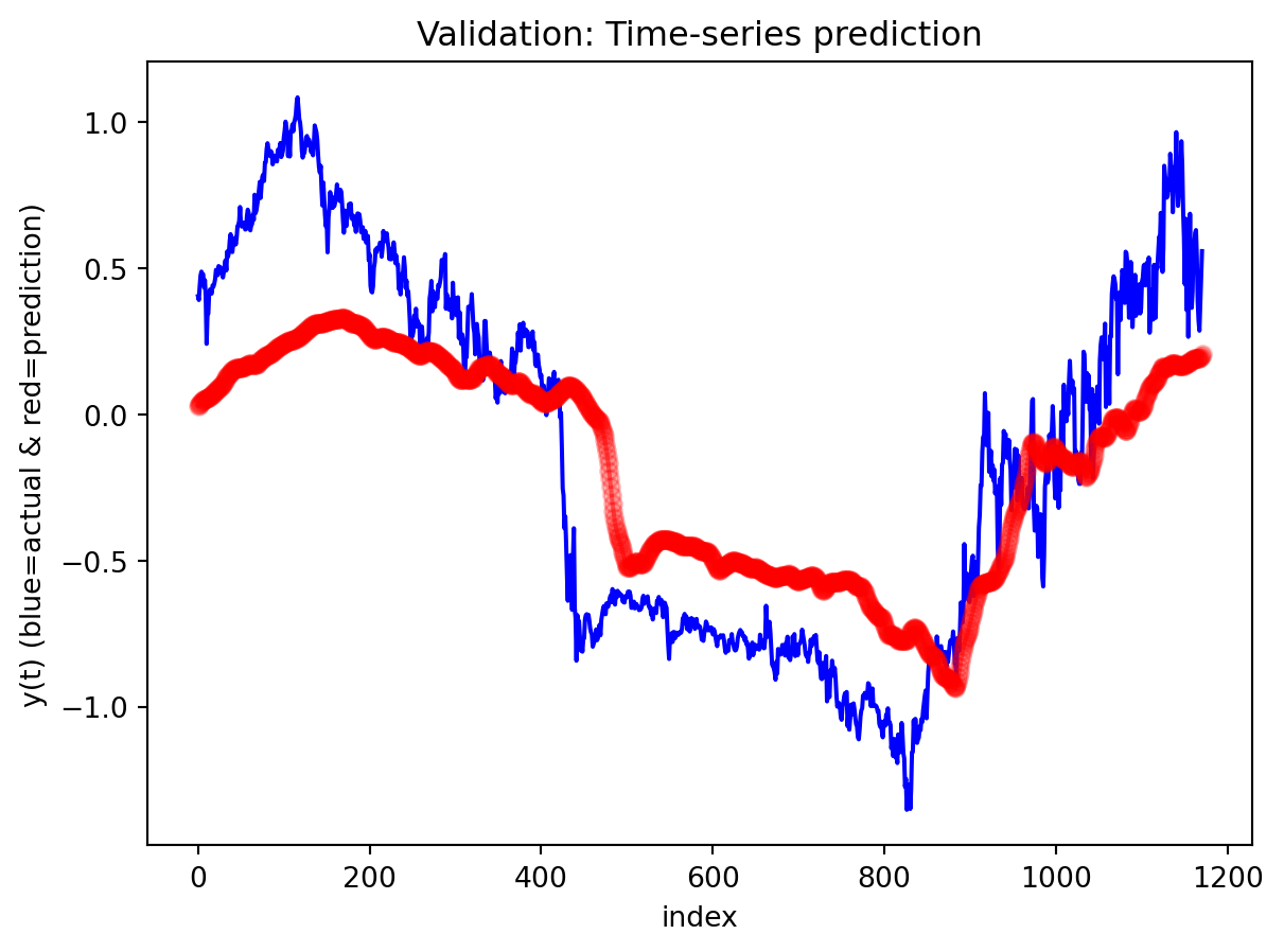
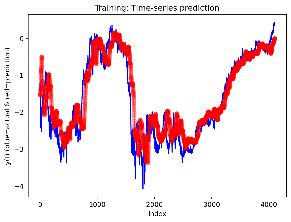
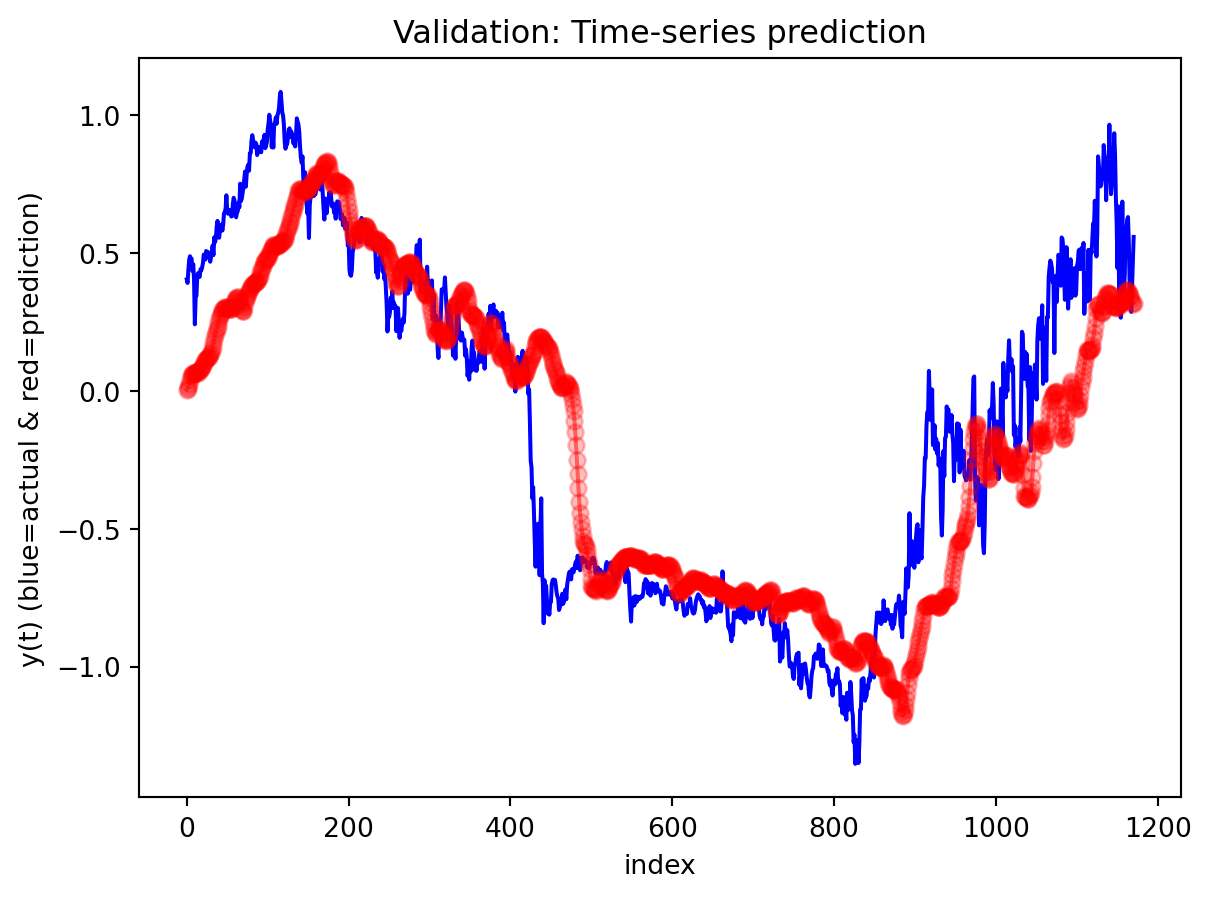
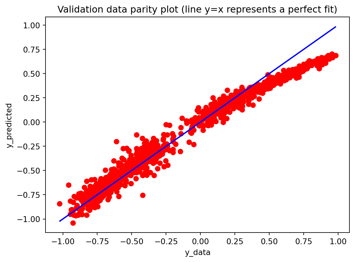
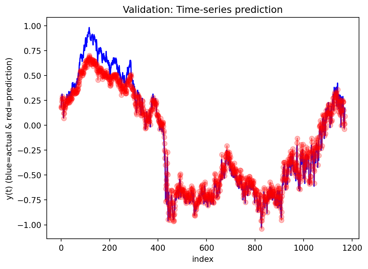
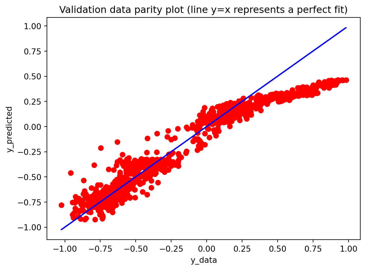
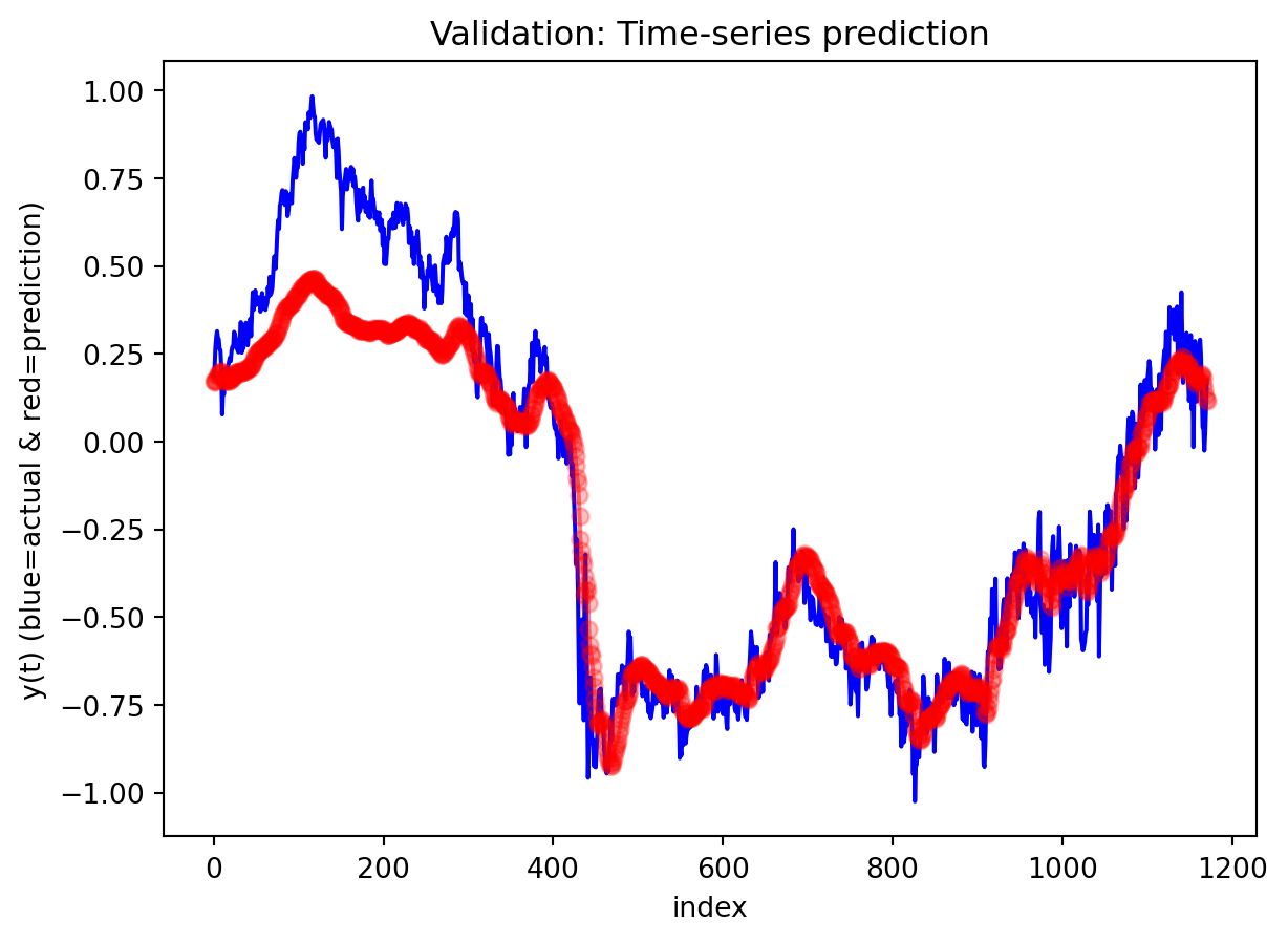
Across both the 3-year and 10-year yield spreads, the simple RNN achieves the lowest RMSE among the three deep learning models, with the GRU second and the LSTM performing worst. However, directional accuracy is only around 40–50% for all models, which is not high enough to consider any of them as strong short-term forecasting tools. This suggests that while the RNN and GRU can track the overall level of the spread reasonably well, they struggle to capture short-horizon fluctuations. The LSTM, despite being the most complex architecture, delivers the highest RMSE and only slightly better directional accuracy for the 3-year spread.
-Effectiveness of Regularization
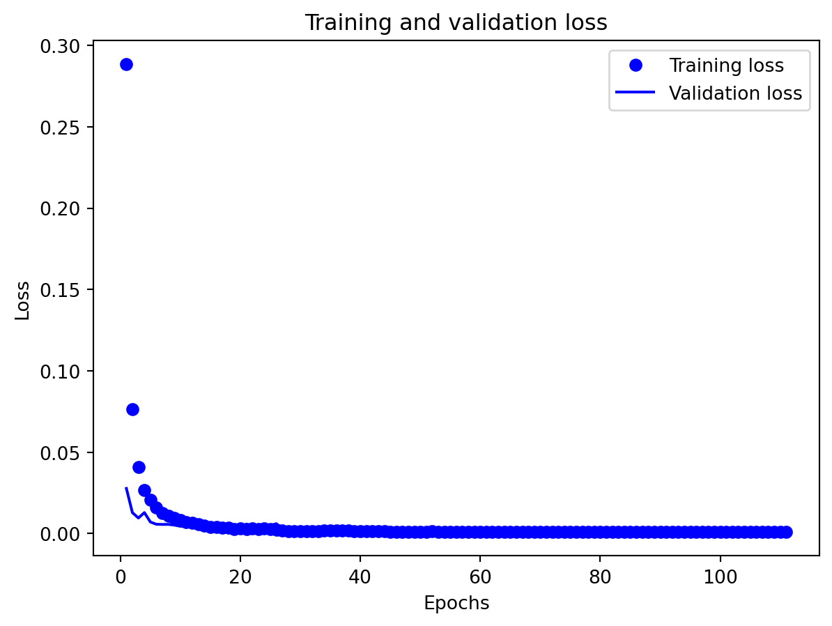
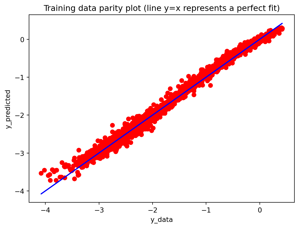
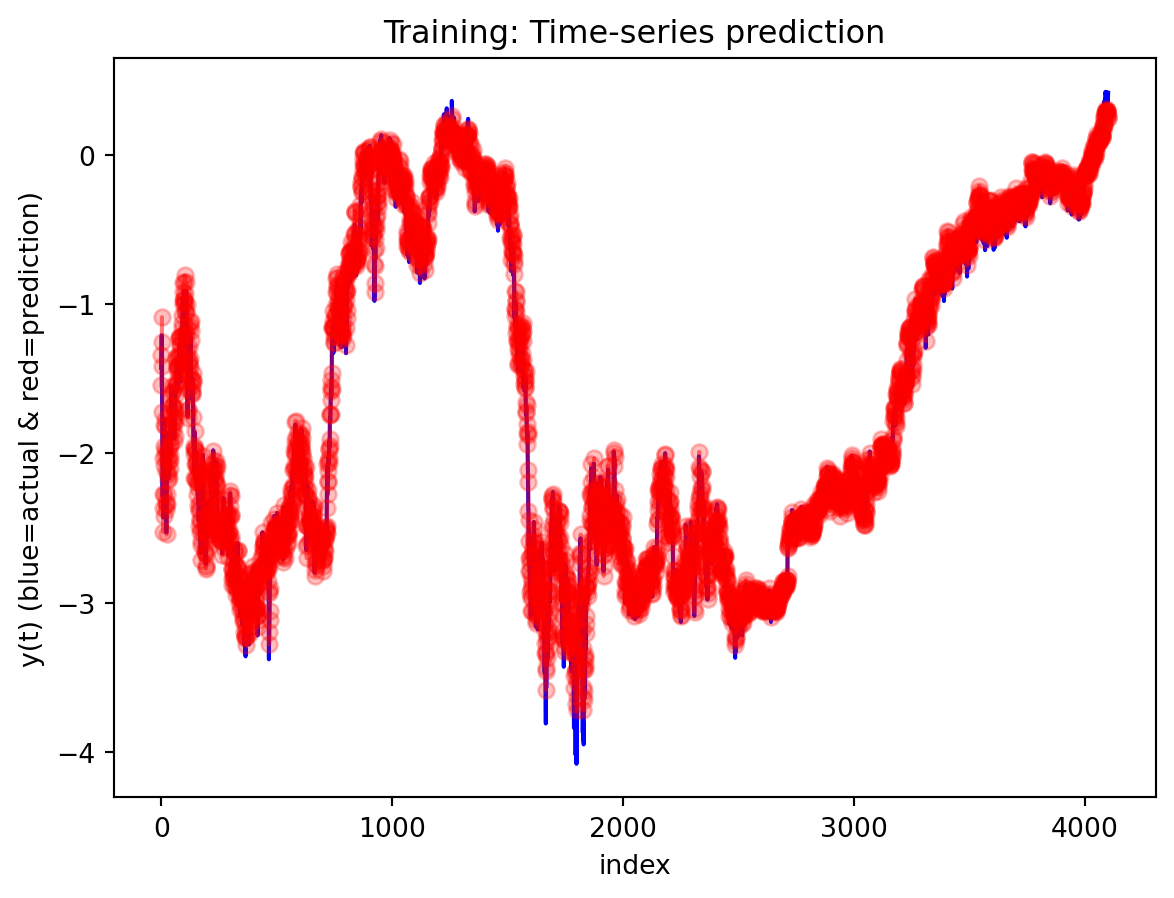
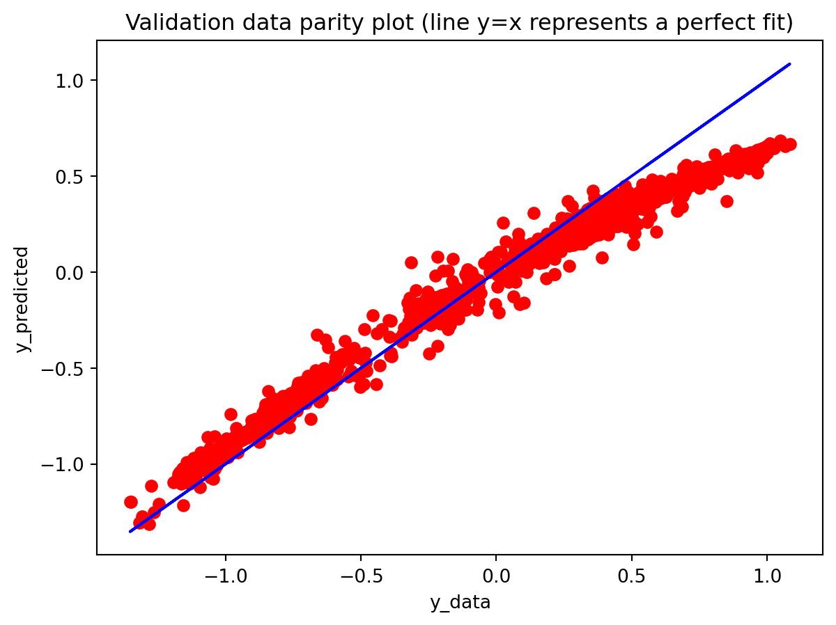
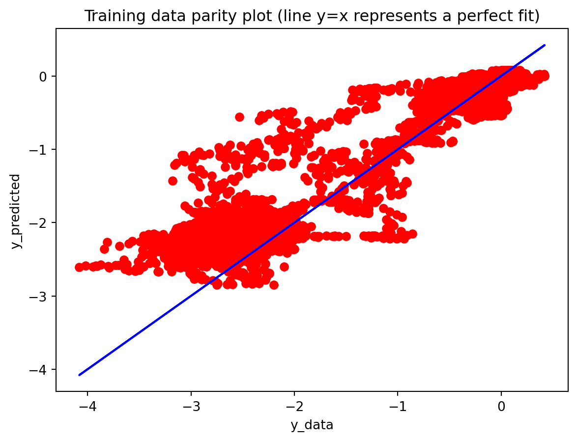
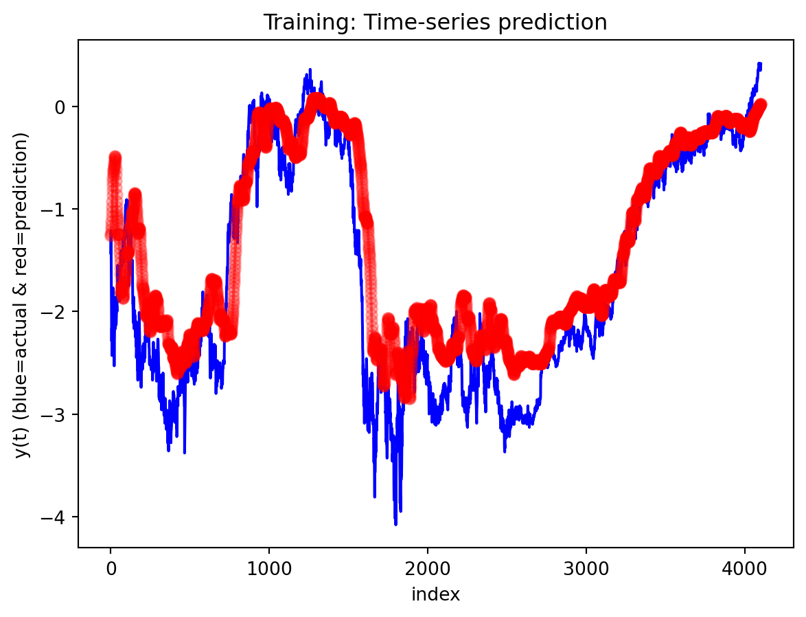
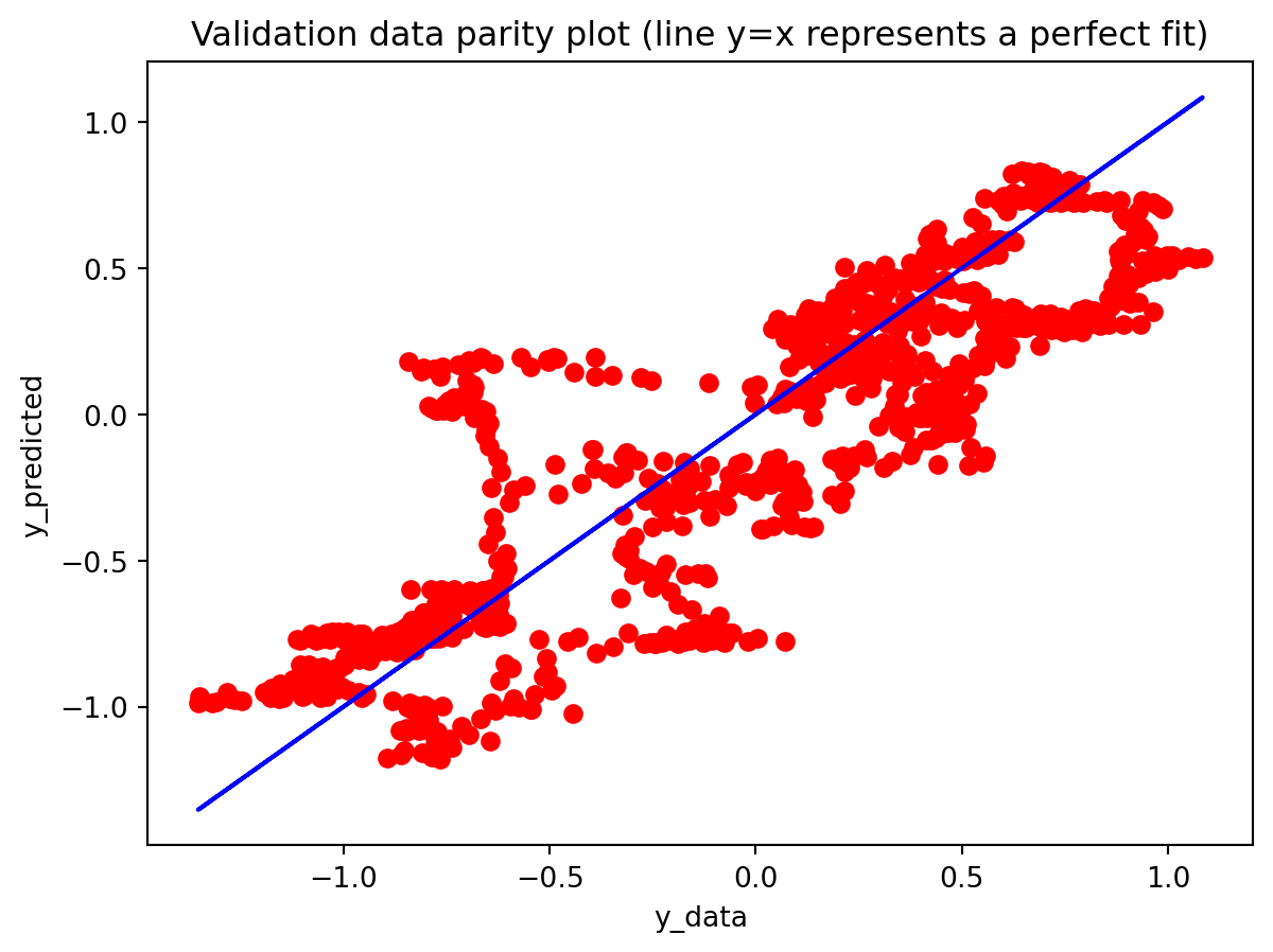
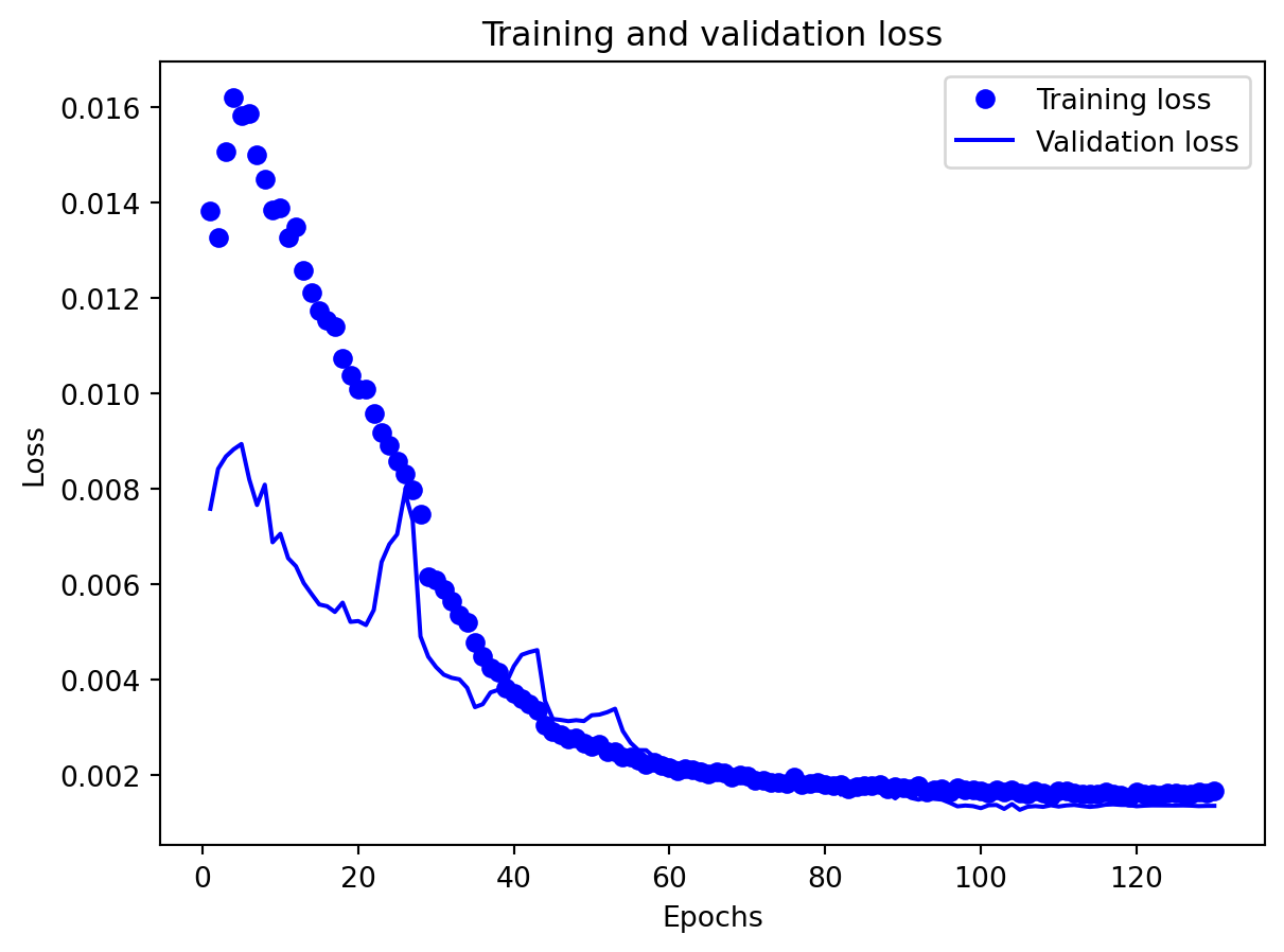
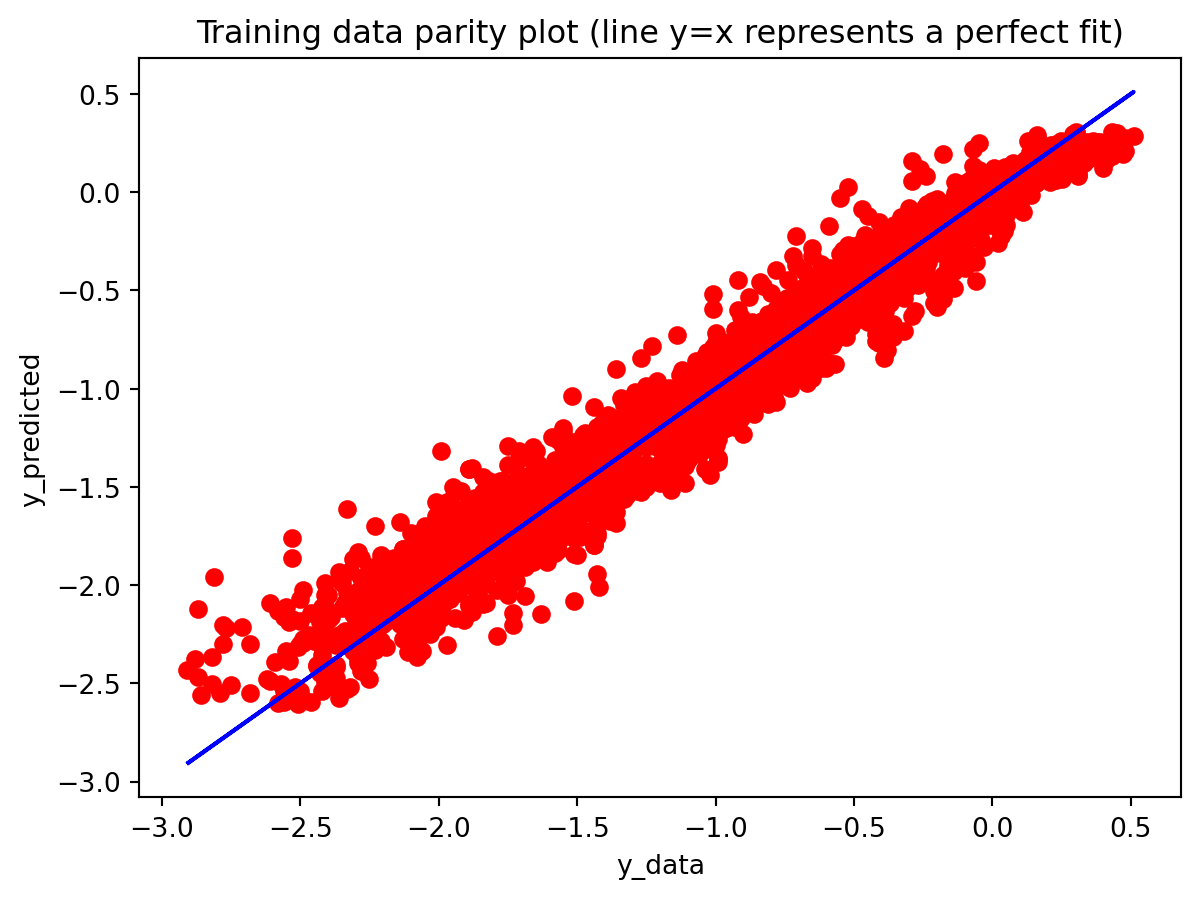
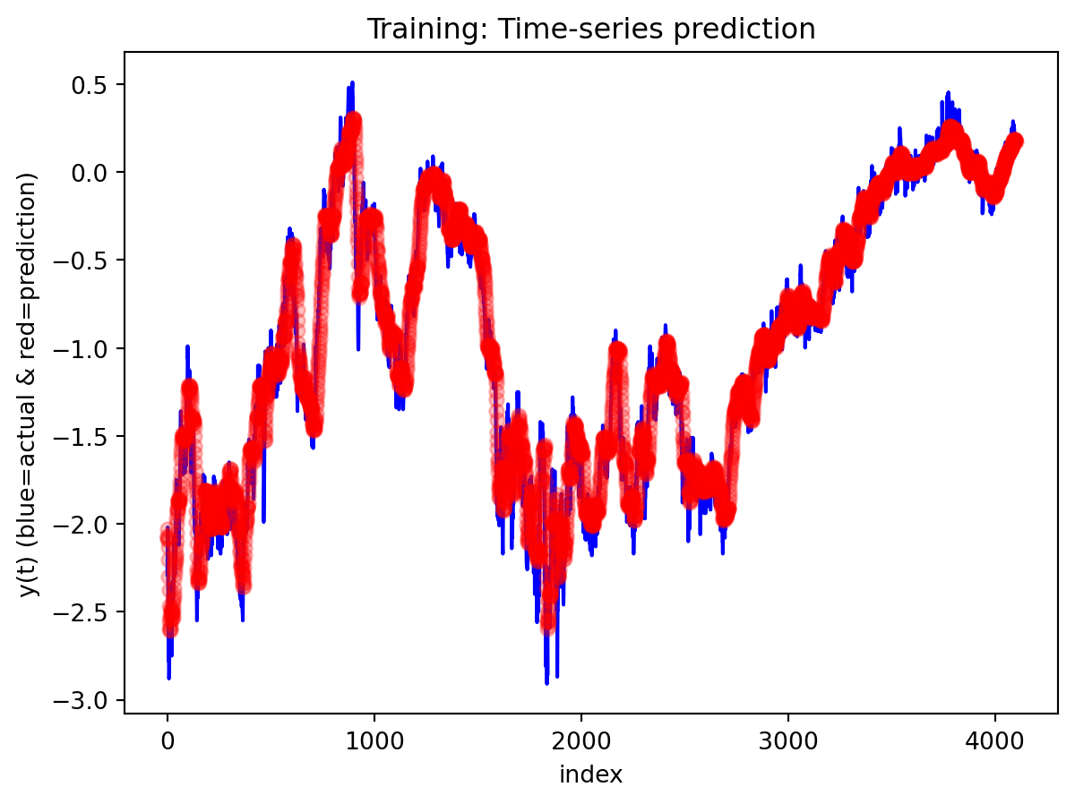
All three architectures are trained under the same regularization scheme: dropout of 0.3 after each layer, early stopping on validation loss with a patience of 25 epochs, and a ReduceLROnPlateau scheduler to lower the learning rate when validation loss stops improving. The training logs indicate that this setup keeps optimization stable and mitigates overfitting. For the 3-year RNN, the final training loss is approximately 0.00081 versus a validation loss of about 0.00093, with early stopping triggered around epoch 79 out of 104. For the 3-year GRU, the training loss is about 0.00143 and the validation loss about 0.00106, again fairly close. The 10-year models show similar behavior; in some cases, the validation loss is even slightly lower than the training loss (e.g., 10Y RNN train 0.00090 vs. val 0.00042), which is consistent with dropout noise and early stopping rather than severe overfitting. The training and validation loss plots support this interpretation. Thus, regularization is effective in maintaining training stability and preventing runaway overfitting, and the gap between training and validation losses is modest for all models. Nevertheless, there remains a clear performance gap between architectures: the LSTM still generalizes worse than the RNN and GRU, suggesting that its complexity is excessive relative to the information contained in a single univariate spread.
-Comparison with Traditional Models
The summary table that compares ARIMA to the deep models makes this even clearer. For both maturities, ARIMA dramatically outperforms all three deep-learning architectures in terms of RMSE. This indicates that the dynamics of the yield spread are still well captured by relatively low-order linear structure. The additional flexibility of RNNs, LSTMs, and GRUs does not translate into better predictions; instead, it increases variance and complicates model tuning. ARIMA also has advantages in interpretability and stability: its AR and MA coefficients can be directly inspected, the propagation of shocks is transparent, and mean-reversion behavior is easy to characterize. Overall, this comparison shows that deep learning models are not always superior to traditional time series models. However, there may still be room to improve deep learning performance through more careful hyperparameter tuning, richer input features, or alternative architectures. Ultimately, selecting an appropriate model is crucial: more complex methods do not necessarily yield better forecasts when the underlying data-generating process and modeling conditions do not justify that complexity.
Best model (10Y): RNN

==================================================
Forecasting with RNN
==================================================
Forecast horizon and behavior
For both the 3Y and 10Y spreads, the RNN is used to generate 30-step-ahead forecasts with a 95% confidence band built from test residuals. In the first several steps after the forecast origin, the model essentially continues the recent pattern of the test data: the predicted spread stays close to the last observed values and lies comfortably within the confidence interval, suggesting that the one-step dynamics are captured reasonably well over a short horizon. As we move further out, however, the behavior changes: the forecast path becomes noticeably smoother than the historical series, sharp day-to-day fluctuations are damped, and the uncertainty band fans out. This is typical of a one-step-ahead model applied recursively—the forecasts are most reliable over roughly the first 10–15 days, after which accumulated errors and the model’s implicit tendency toward a smoothed mean-reverting trajectory dominate. In practice, this means the univariate RNN forecasts are informative for very short-term spread scenarios, while longer-horizon projections should be treated more as indicative trend scenarios with wide uncertainty rather than precise point predictions.
LOOKBACK =30results_exports_rnn = train_single_model(df4, 'RNN', 'South korea Exports to USA(thousand dollars)', LOOKBACK)
############################################################
# South korea Exports to USA(thousand dollars) - RNN
############################################################

Total samples: 361
X shape: (361, 31, 4), y shape: (361, 1)
Train: 252, Val: 72, Test: 37
==================================================
Training RNN...
Parameters: 32,513
==================================================
Training completed in 4.85s
Epochs trained: 29
Best epoch: 4
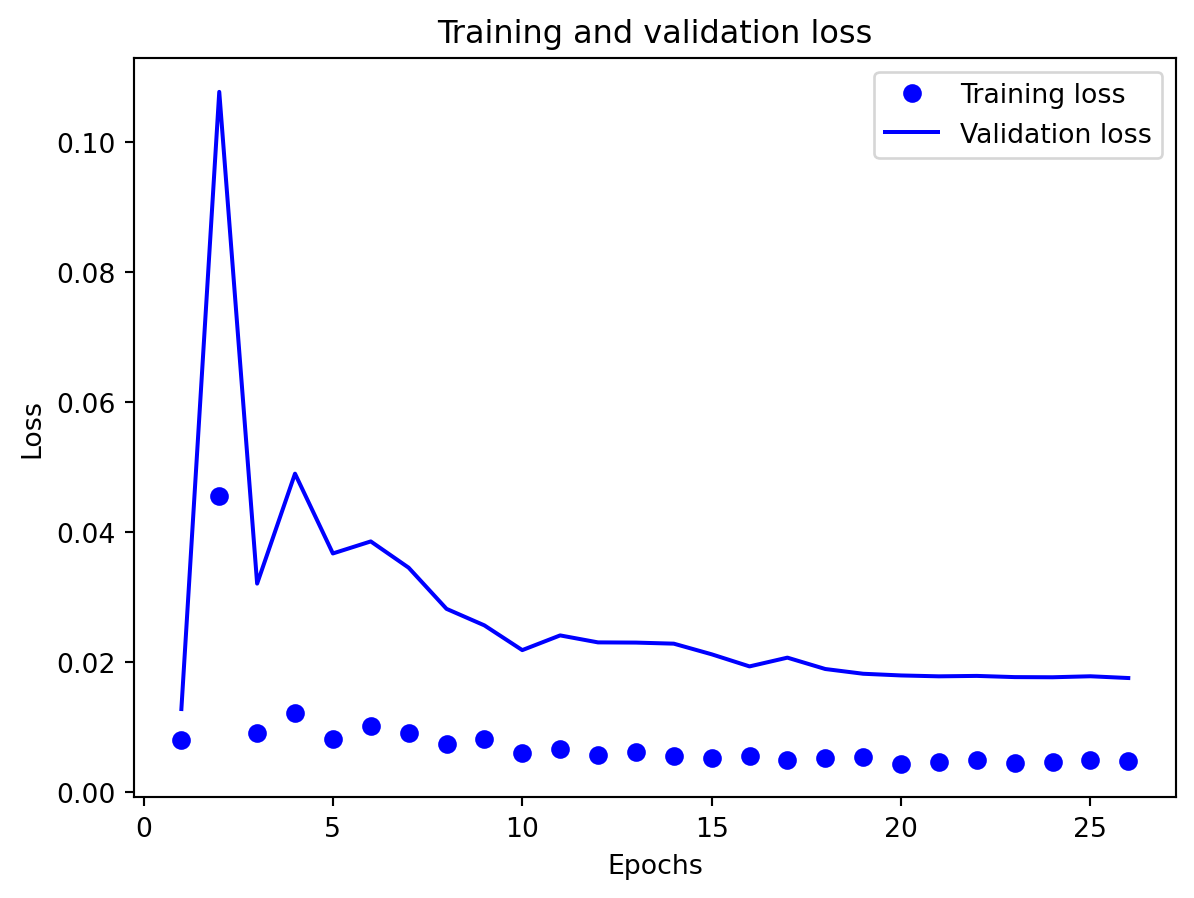
Final train loss: 0.210741
Final val loss: 0.032729
results_exports_lstm = train_single_model(df4, 'LSTM', 'South Korea to USA(thousand dollars)', LOOKBACK)
############################################################
# South Korea to USA(thousand dollars) - LSTM
############################################################

Total samples: 361
X shape: (361, 31, 4), y shape: (361, 1)
Train: 252, Val: 72, Test: 37
==================================================
Training LSTM...
Parameters: 129,953
==================================================
 Training completed in 15.46s
  Epochs trained: 47
  Best epoch: 22
  Final train loss: 0.003109
  Final val loss: 0.006217
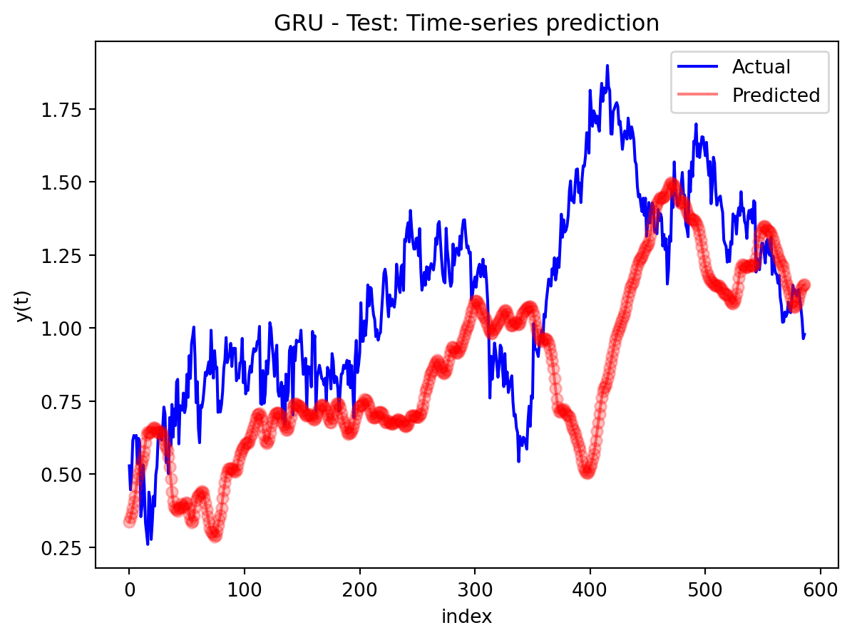
results_exports_gru = train_single_model(df4, 'GRU', 'South Korea export to USA(thousand dollars)', LOOKBACK)
############################################################
# South Korea export to USA(thousand dollars) - GRU
############################################################

Total samples: 361
X shape: (361, 31, 4), y shape: (361, 1)
Train: 252, Val: 72, Test: 37
==================================================
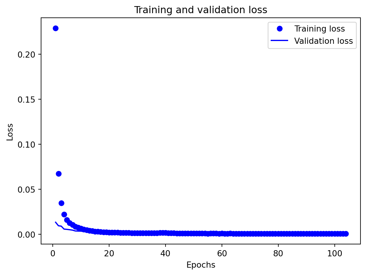
Training GRU...
Parameters: 98,145
==================================================
Training completed in 9.02s
Epochs trained: 26
Best epoch: 1
Final train loss: 0.004761
Final val loss: 0.017573
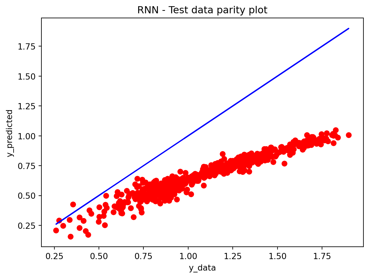
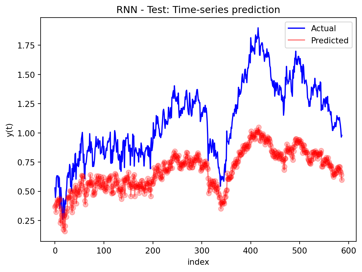
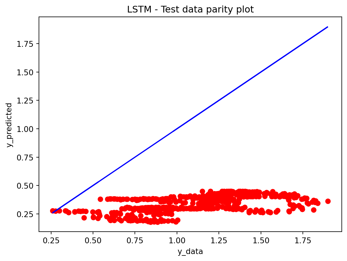
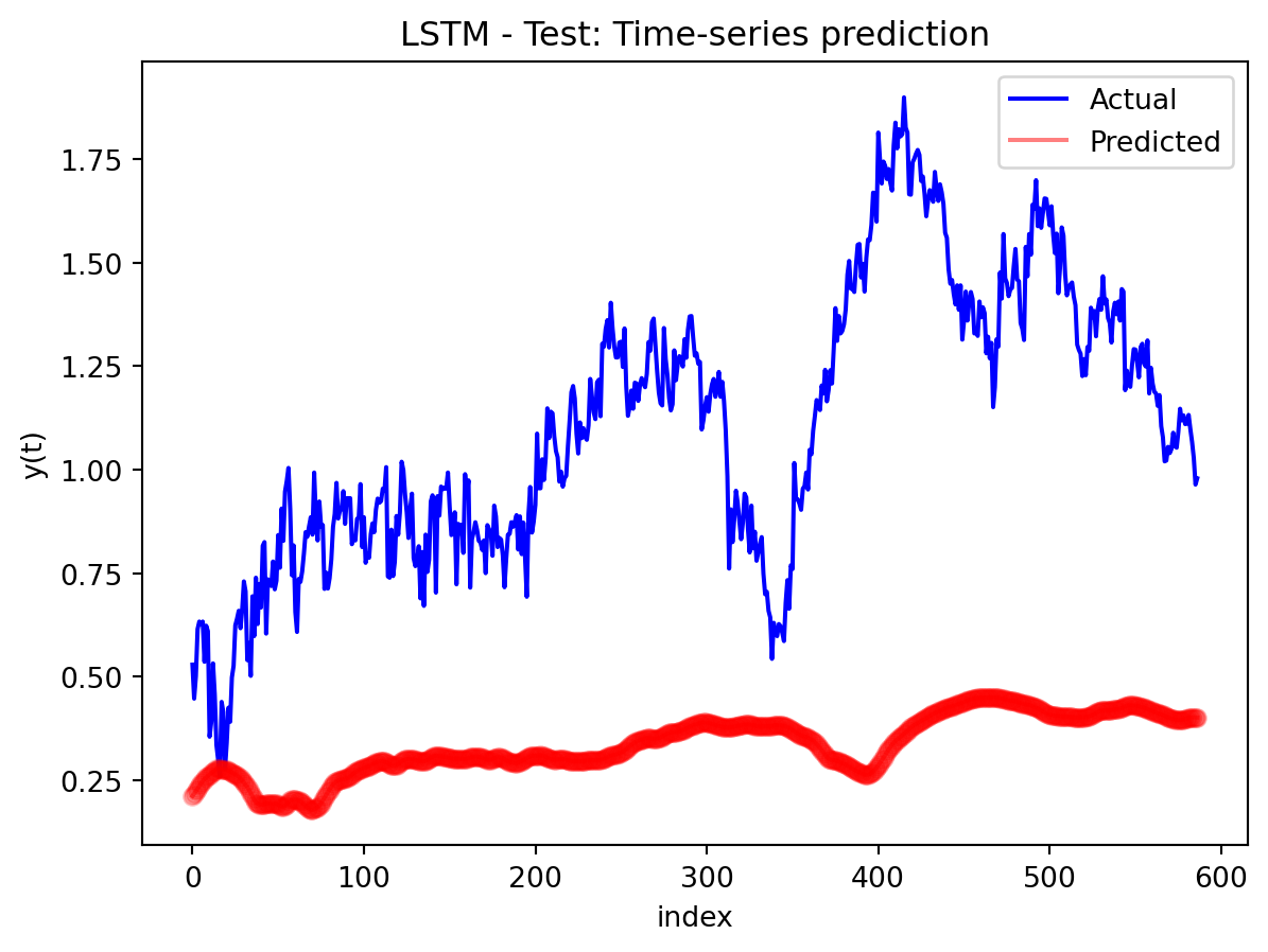
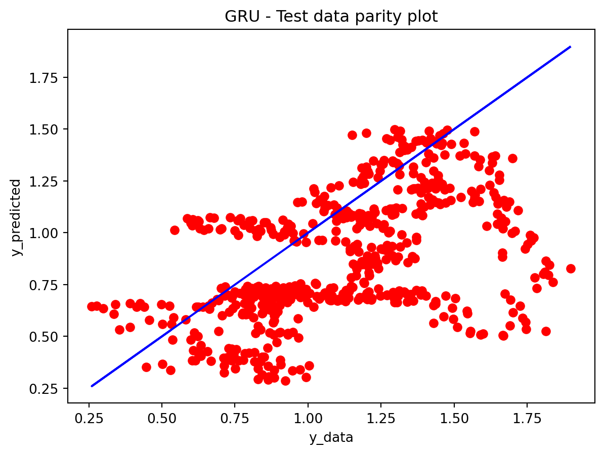
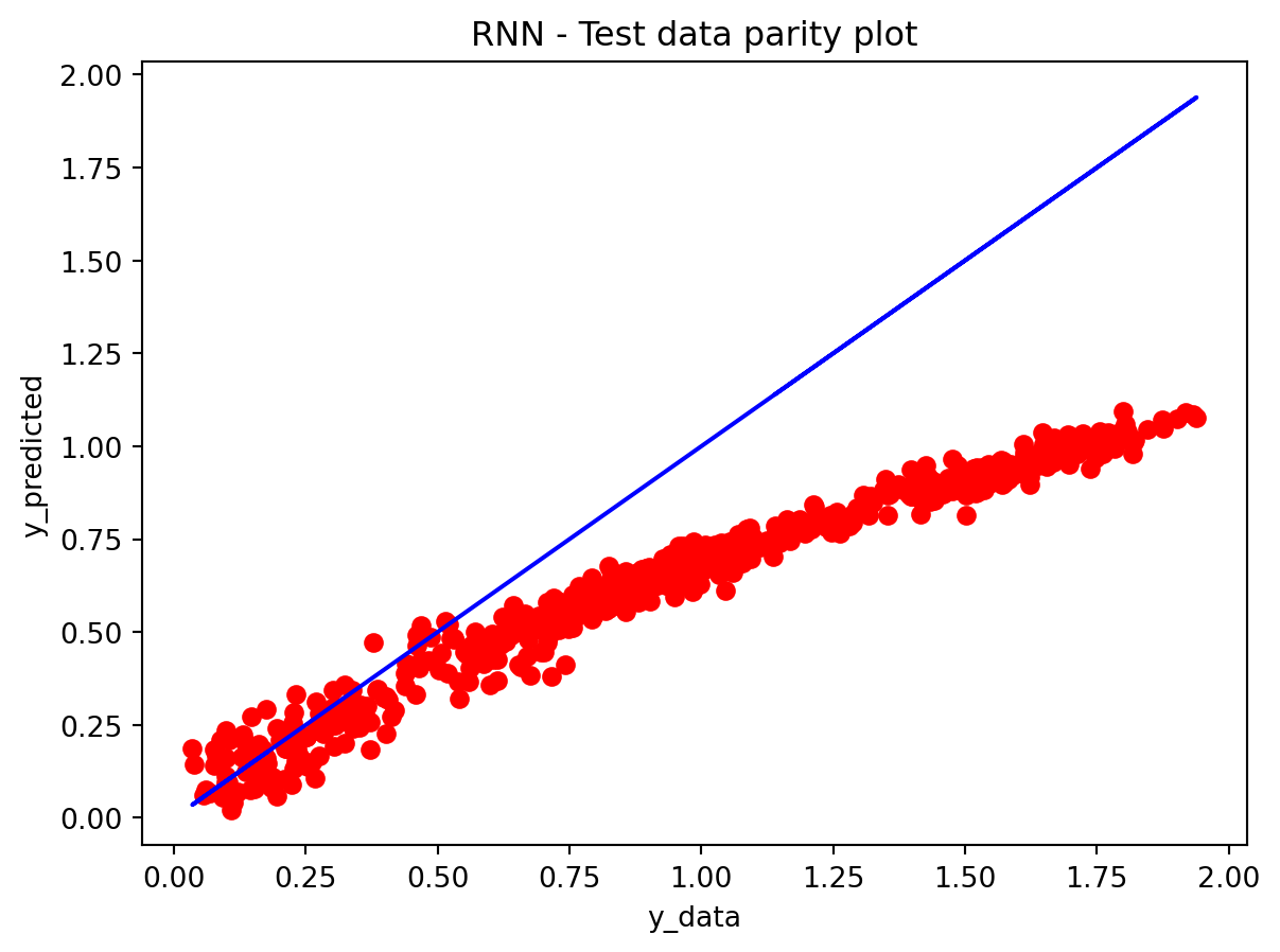
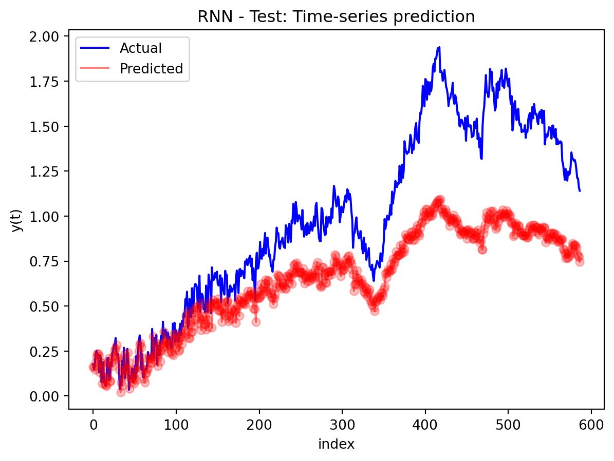
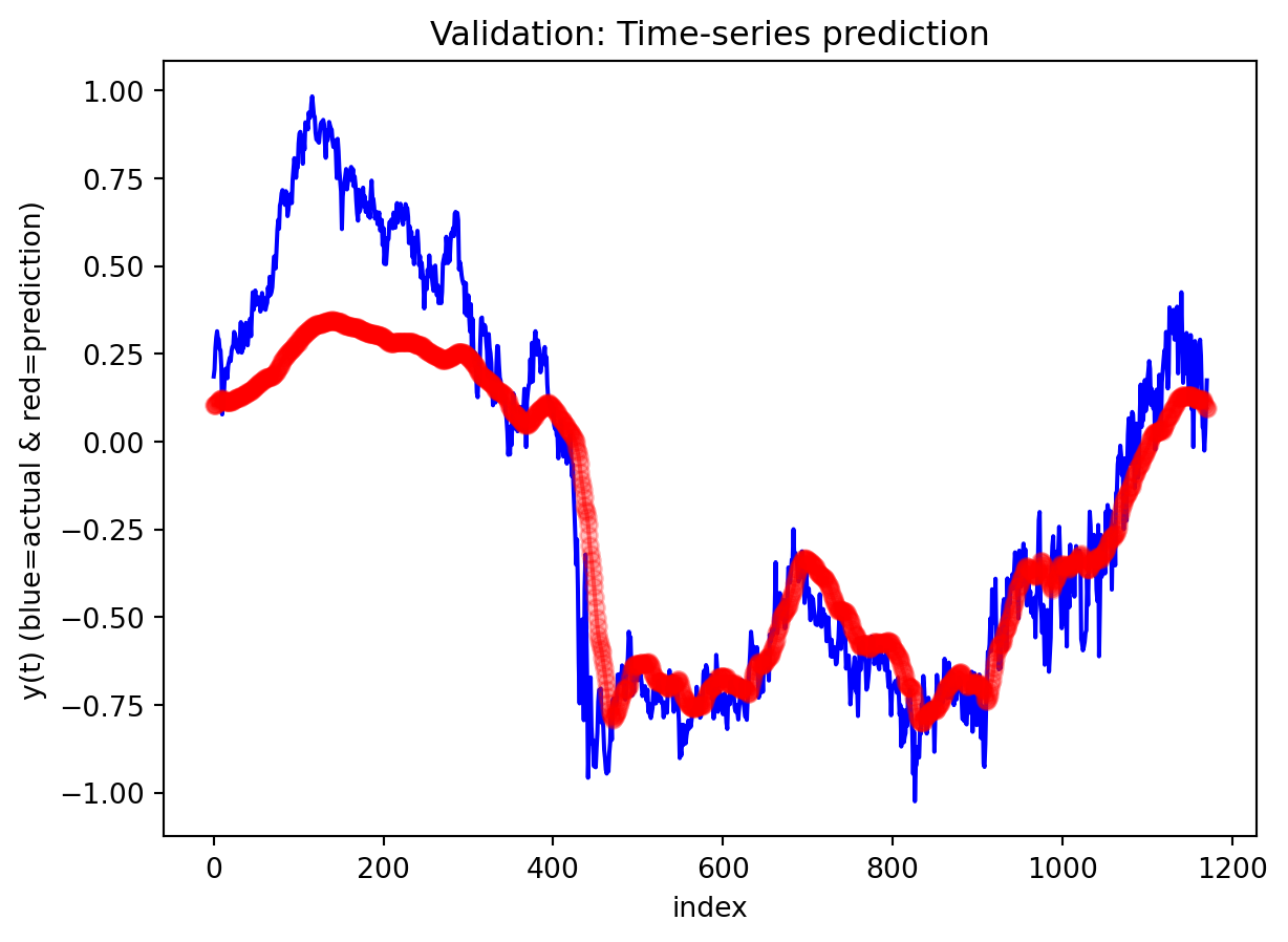
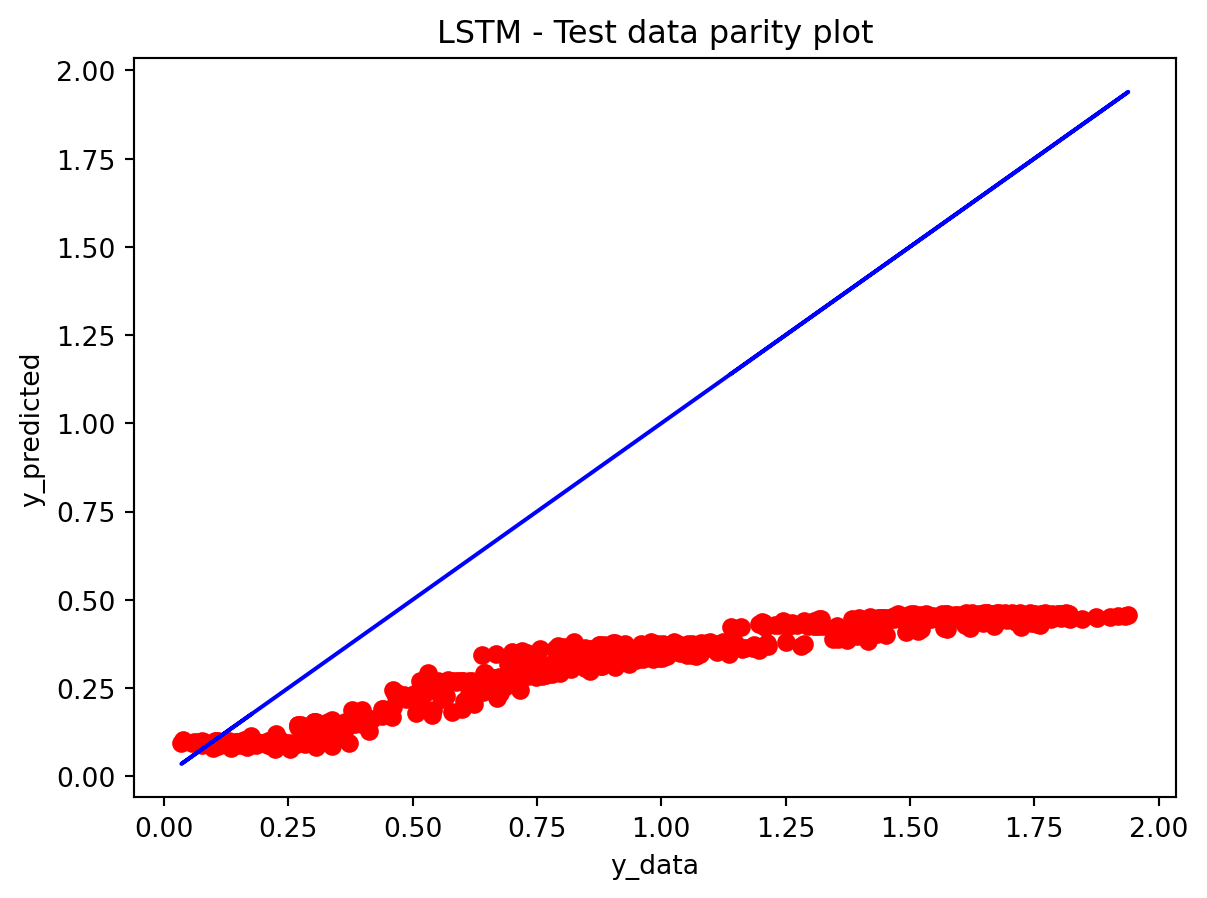
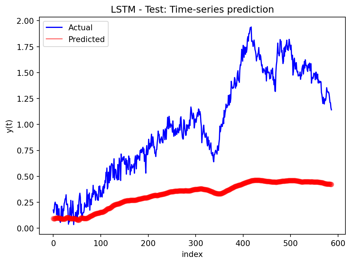
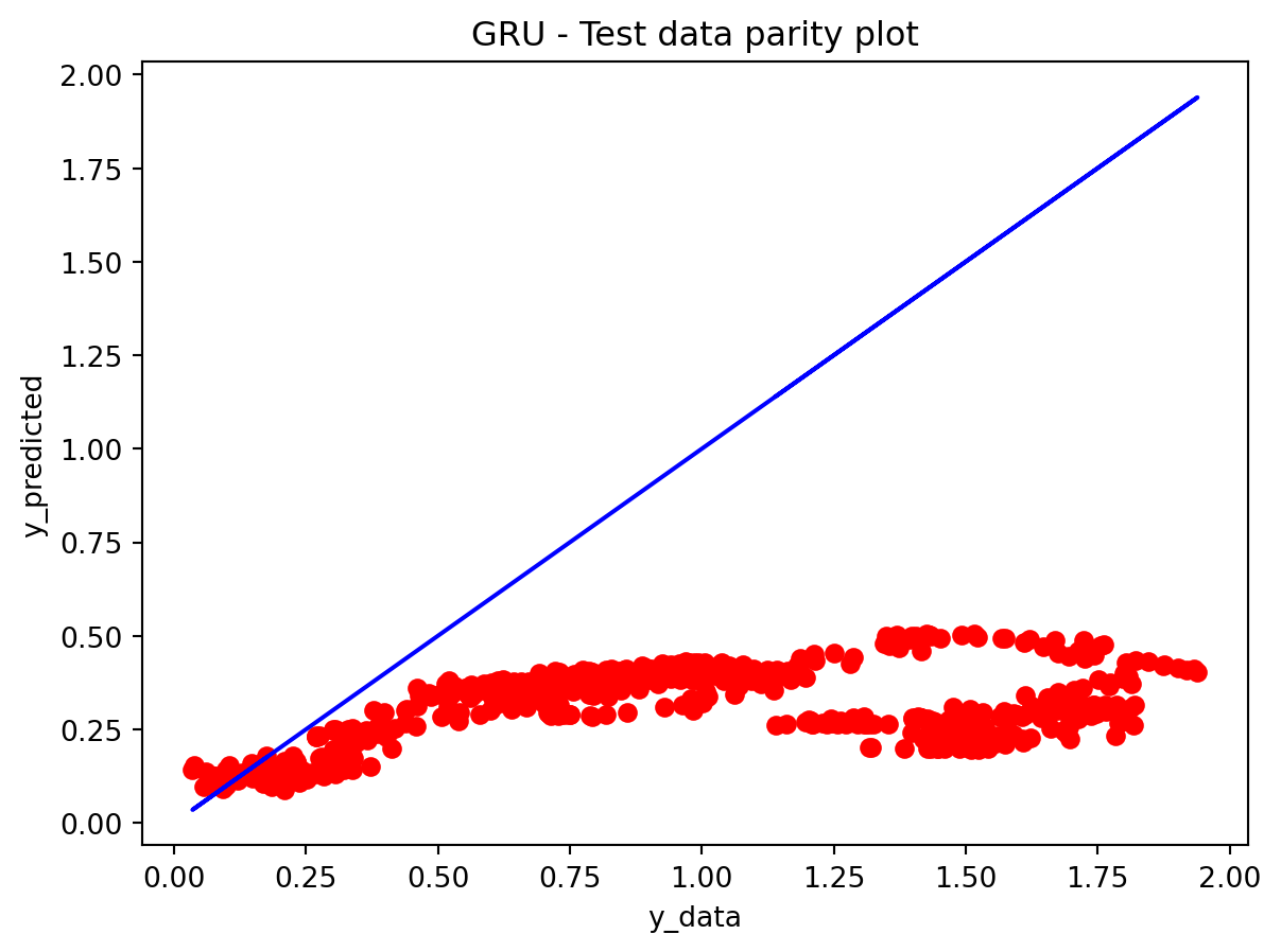
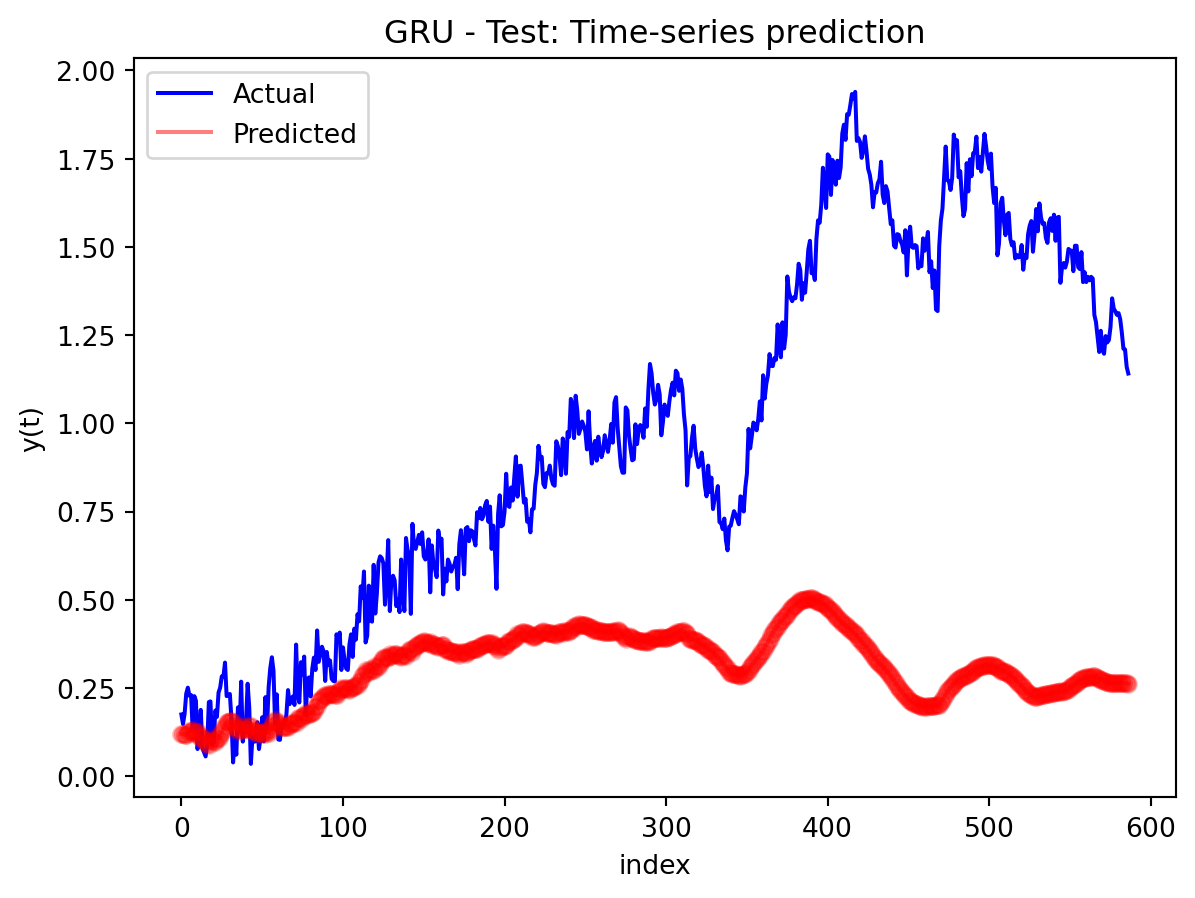
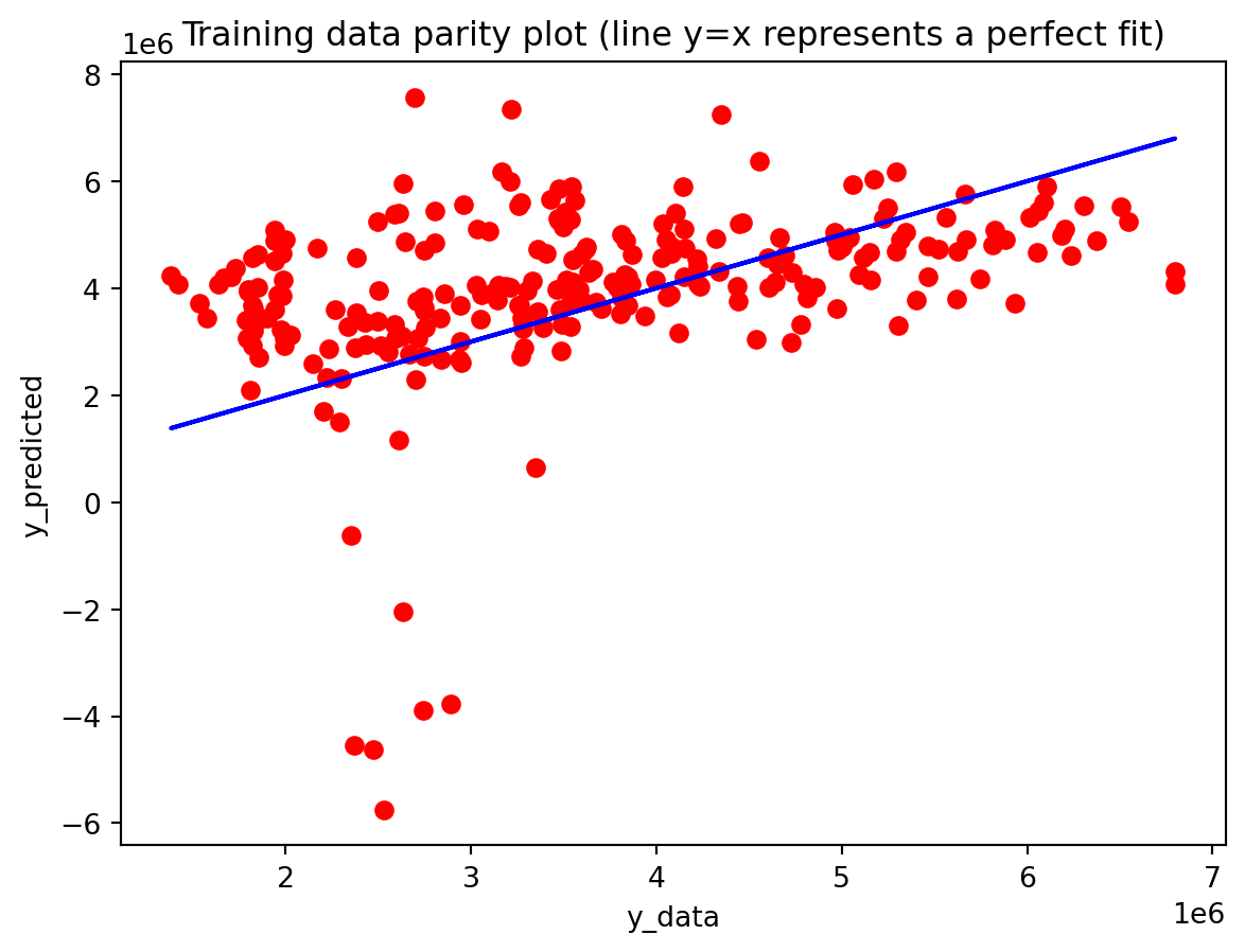
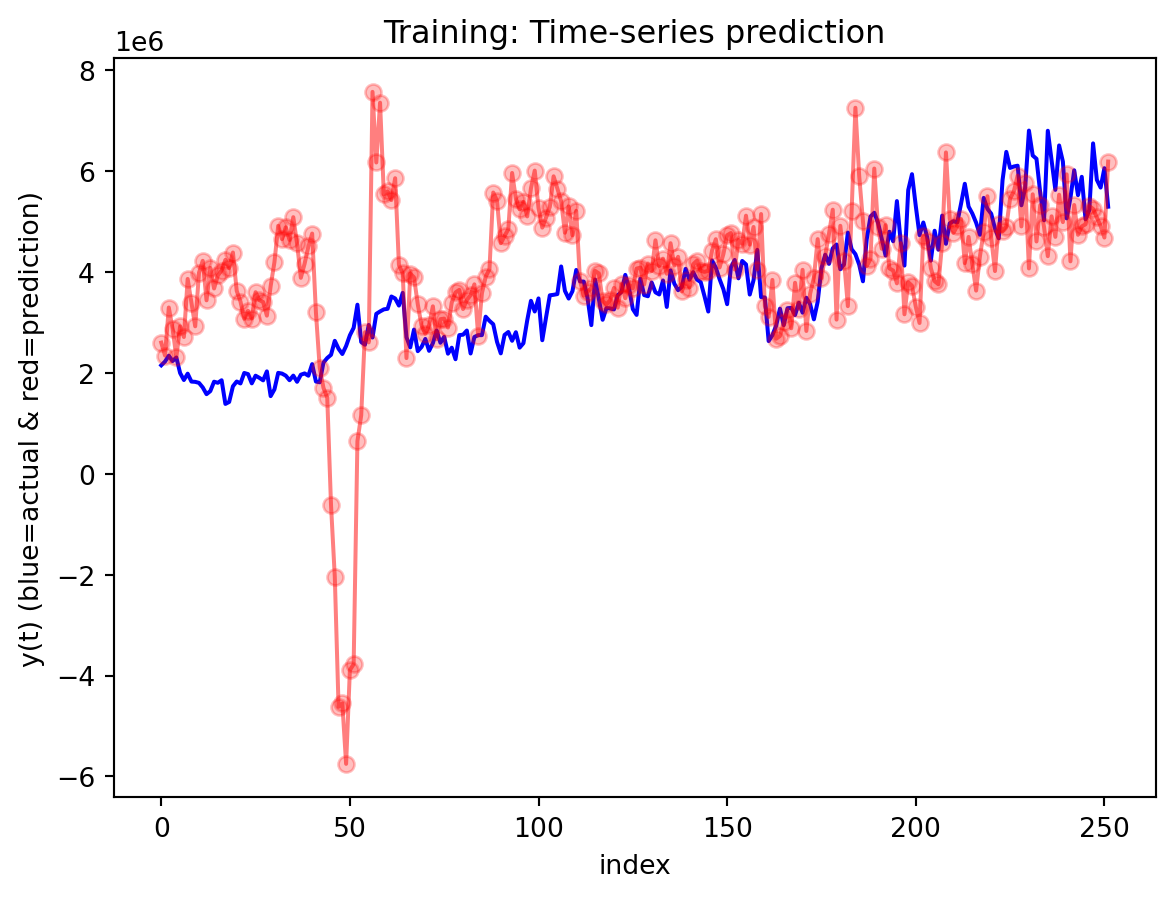
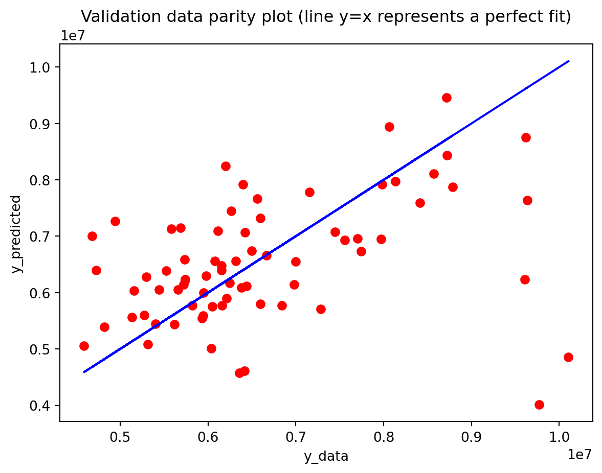
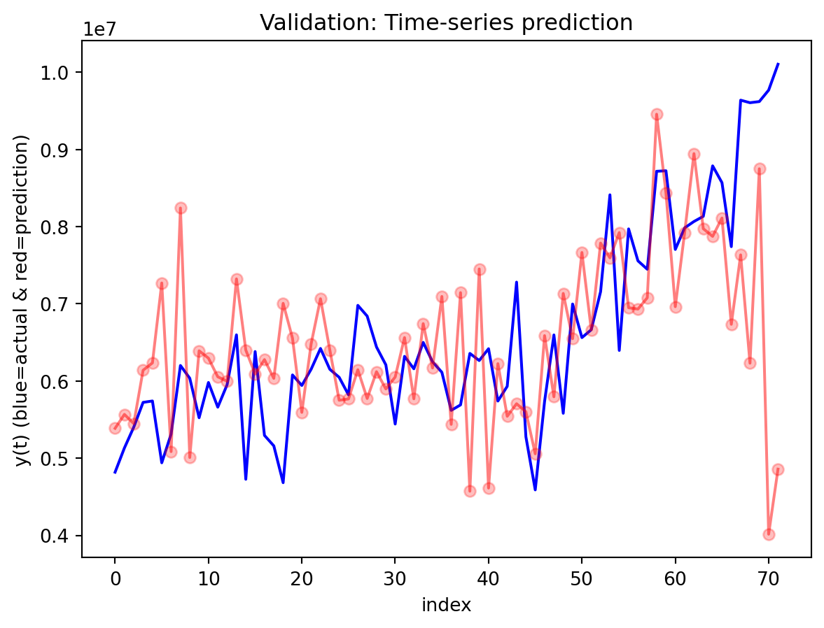
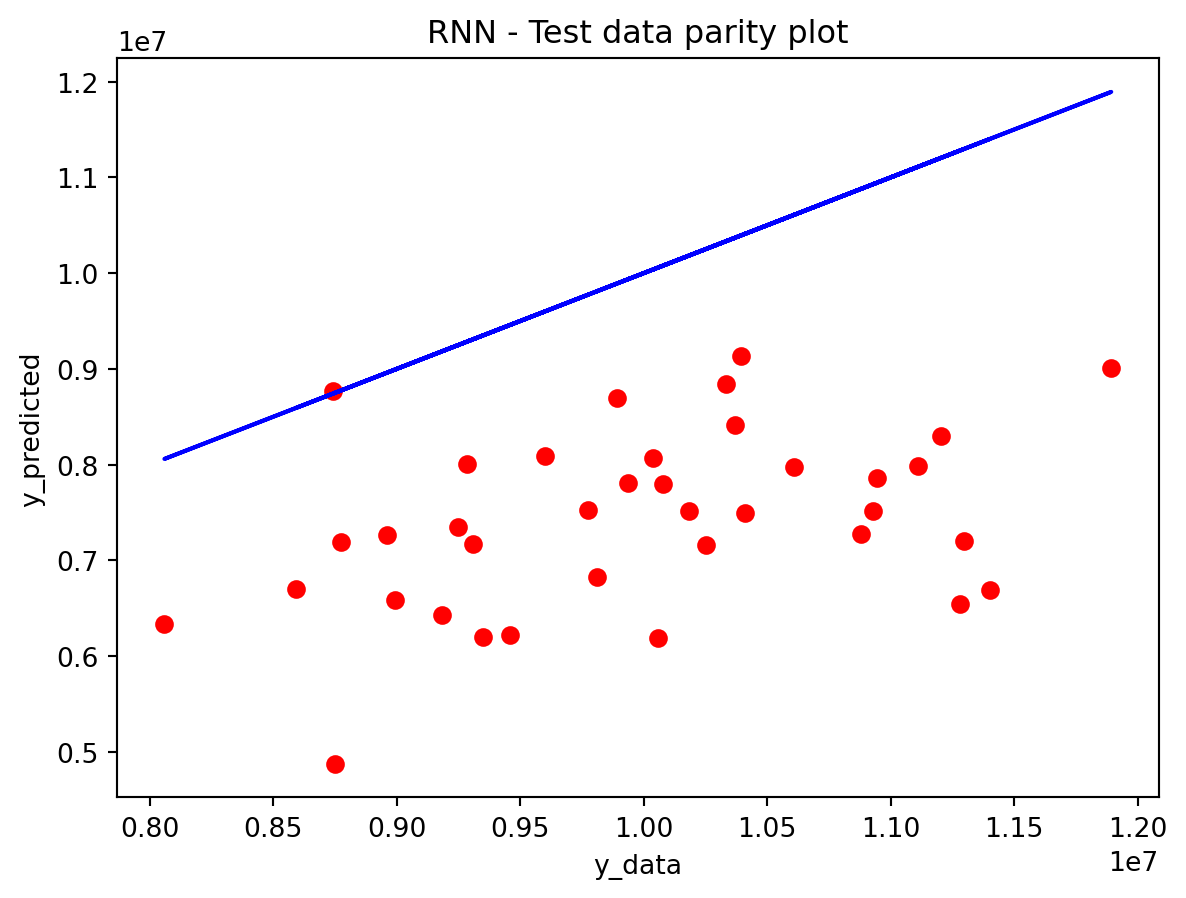
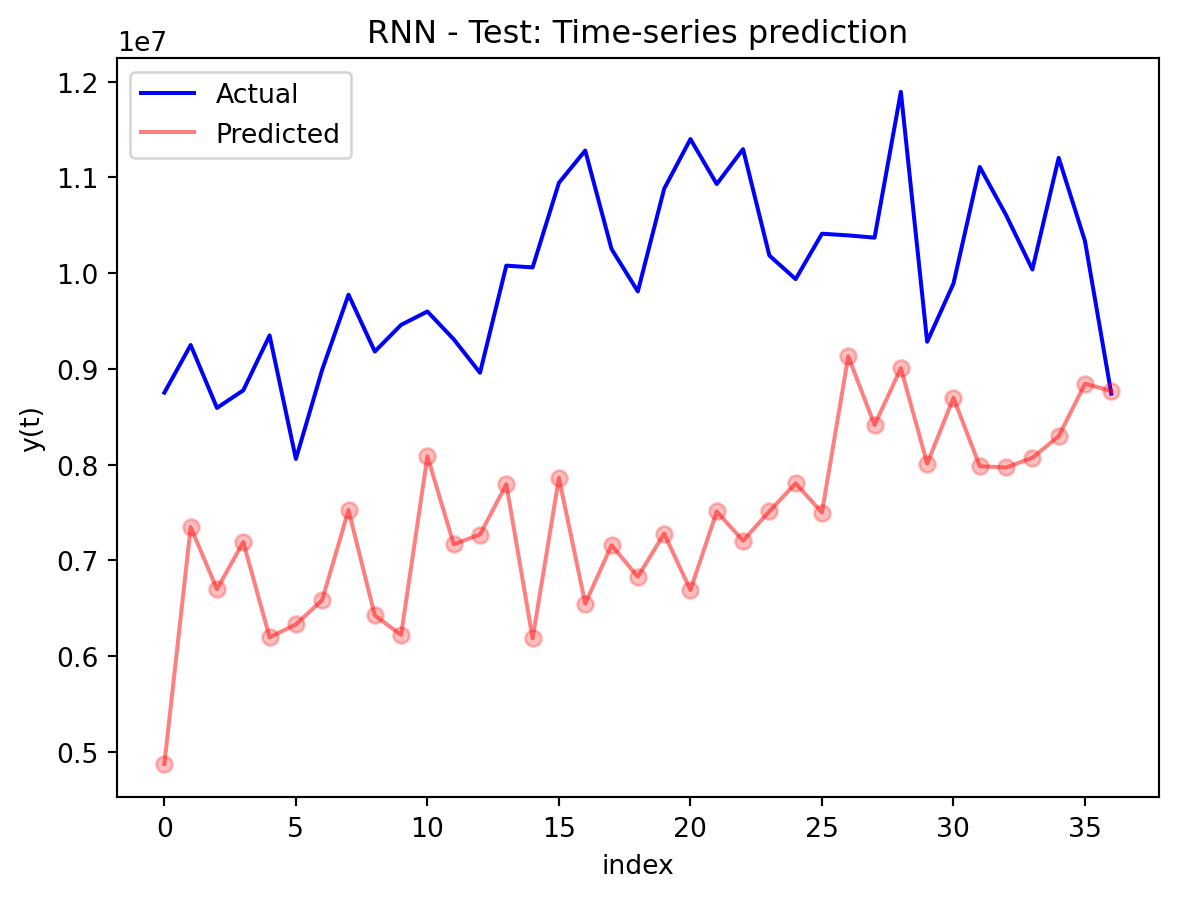
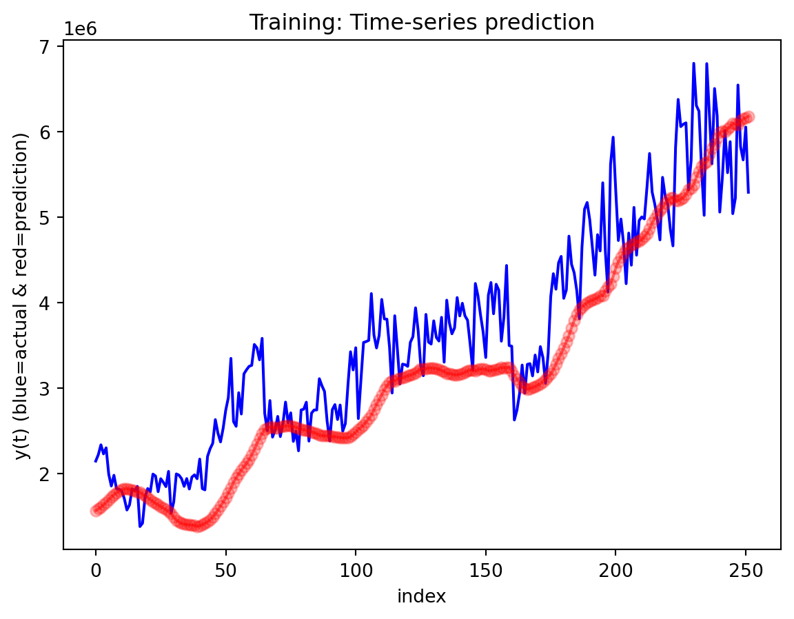
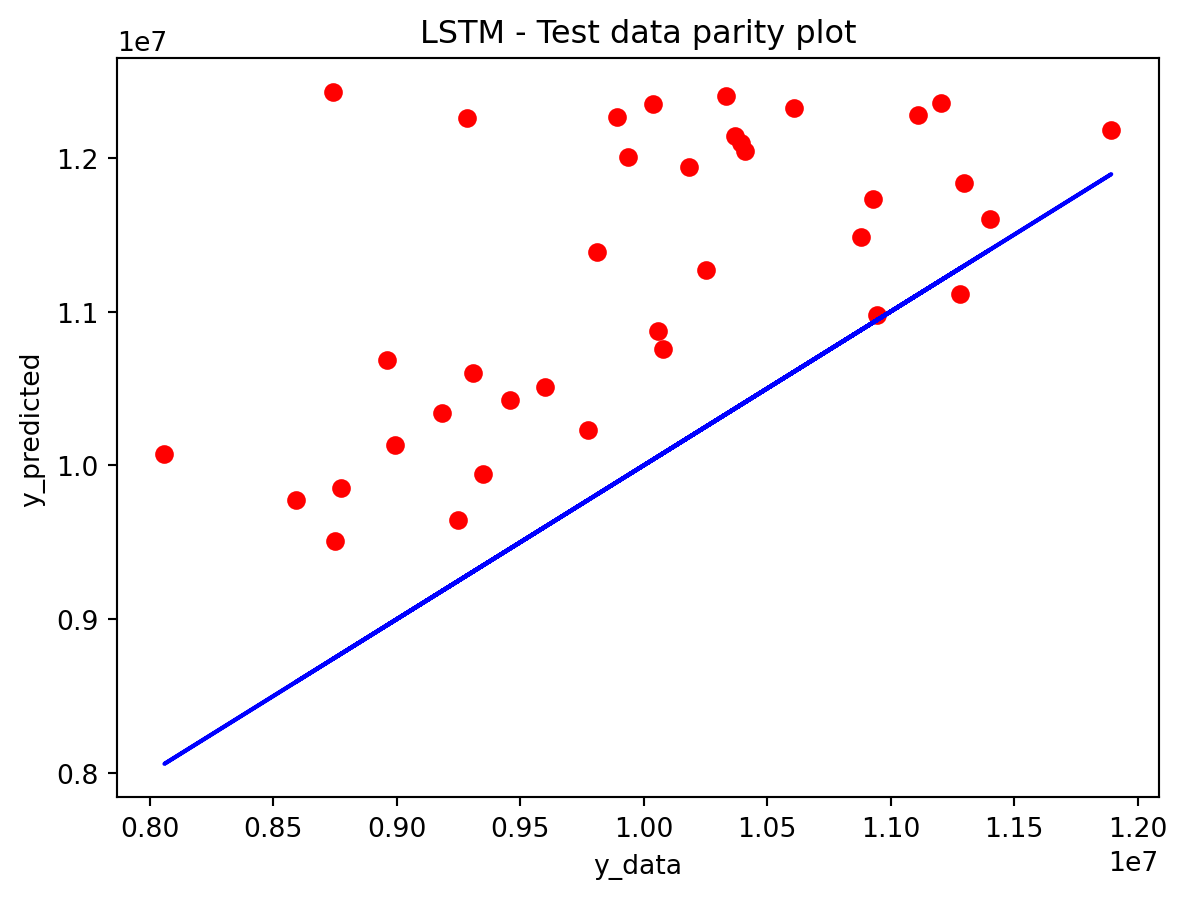
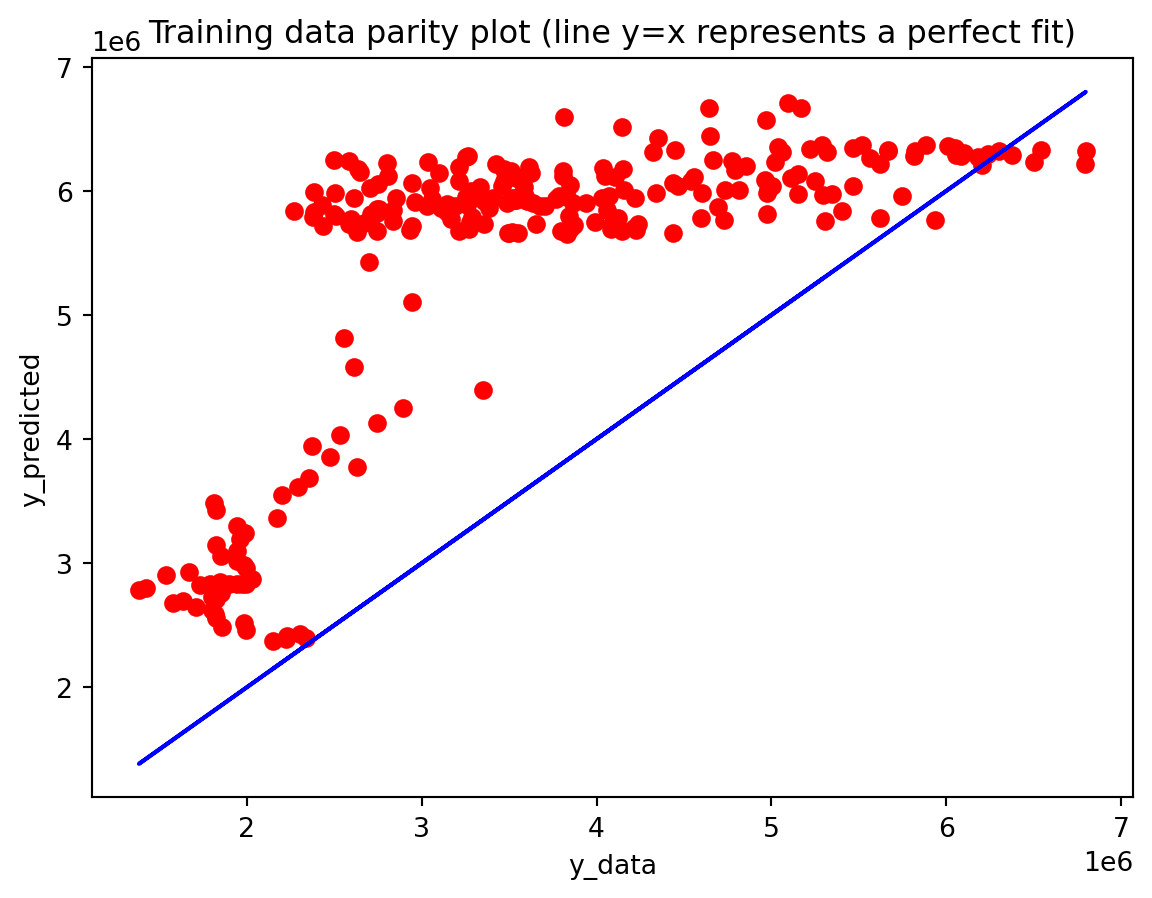
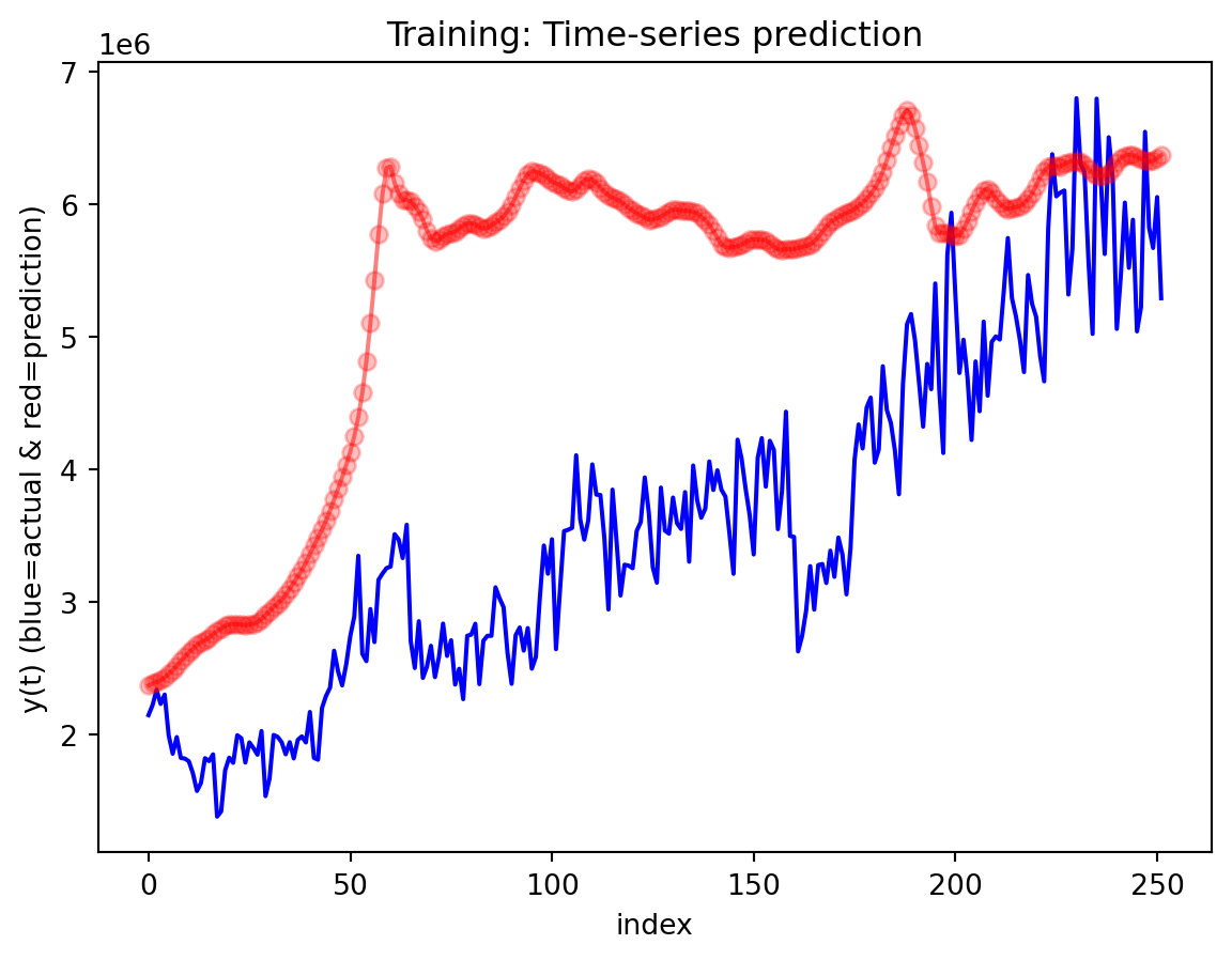
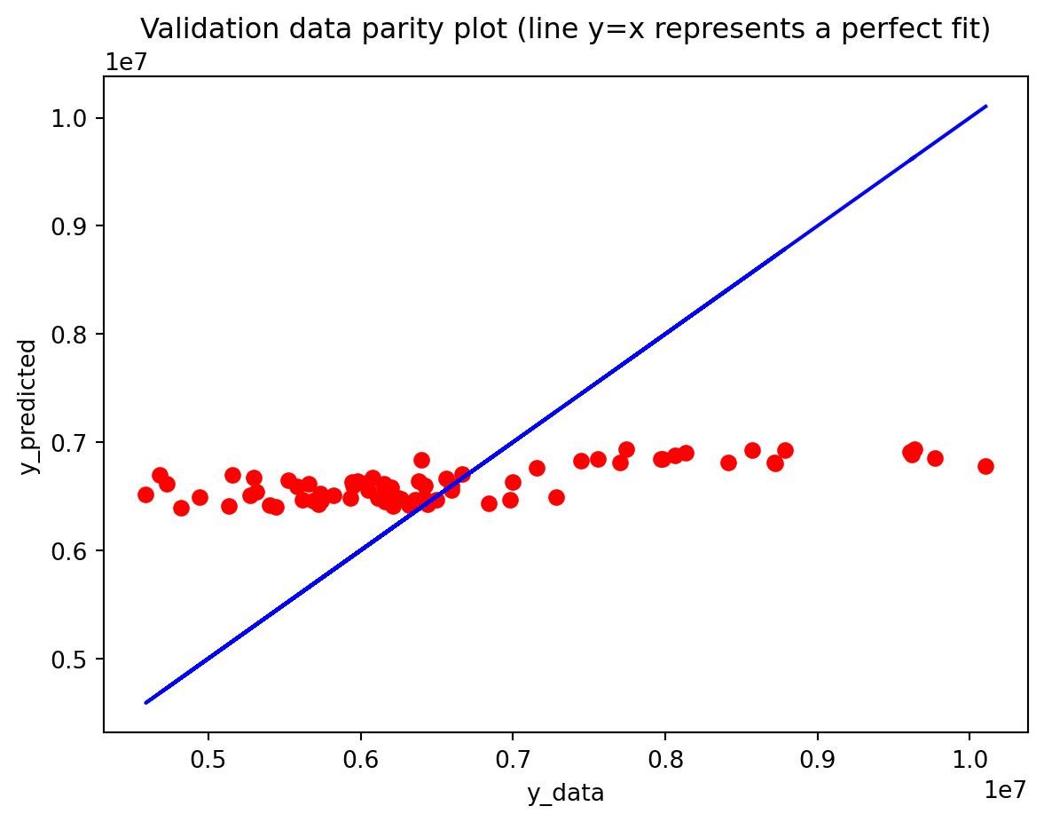
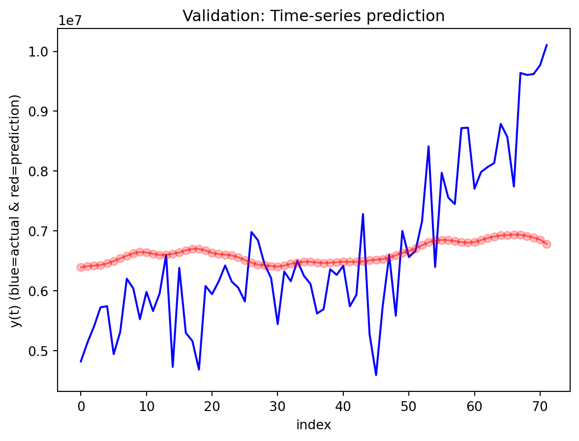
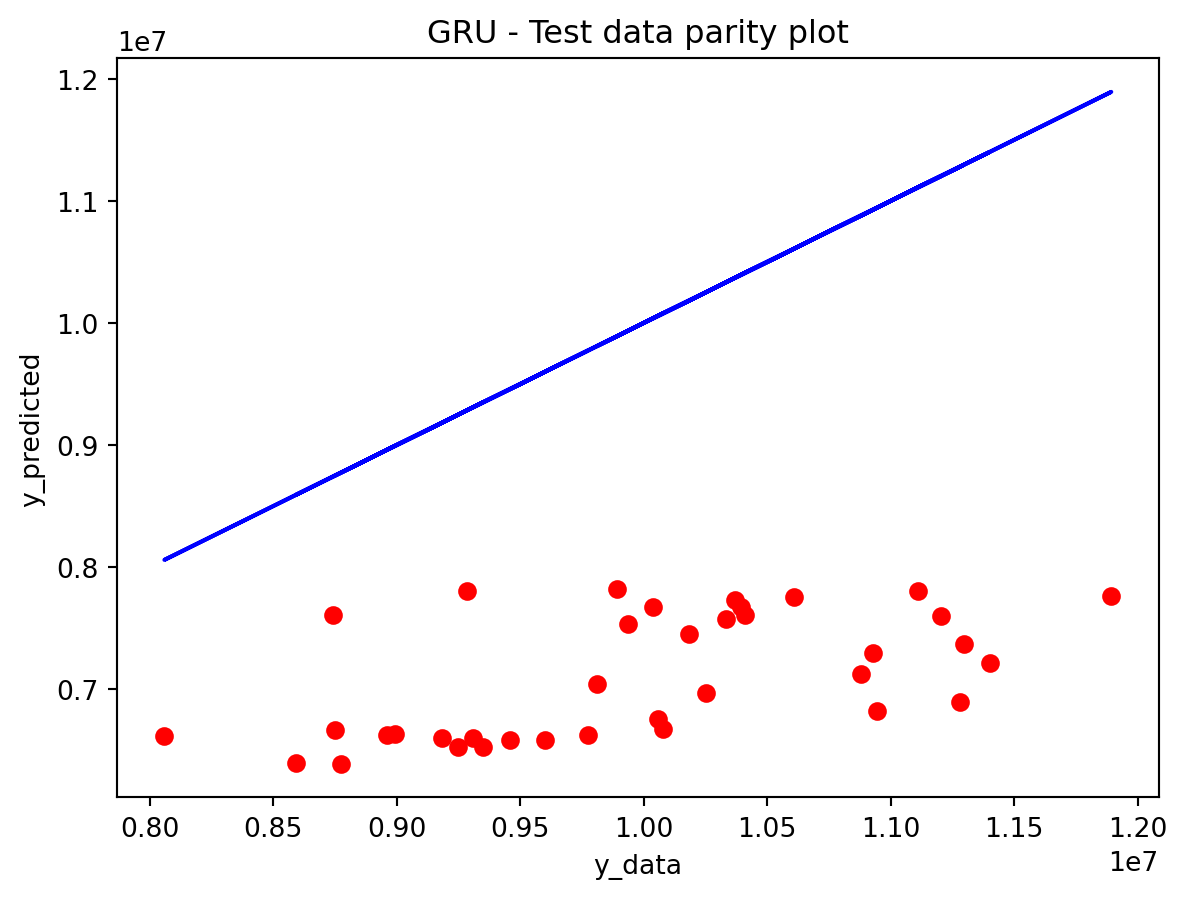
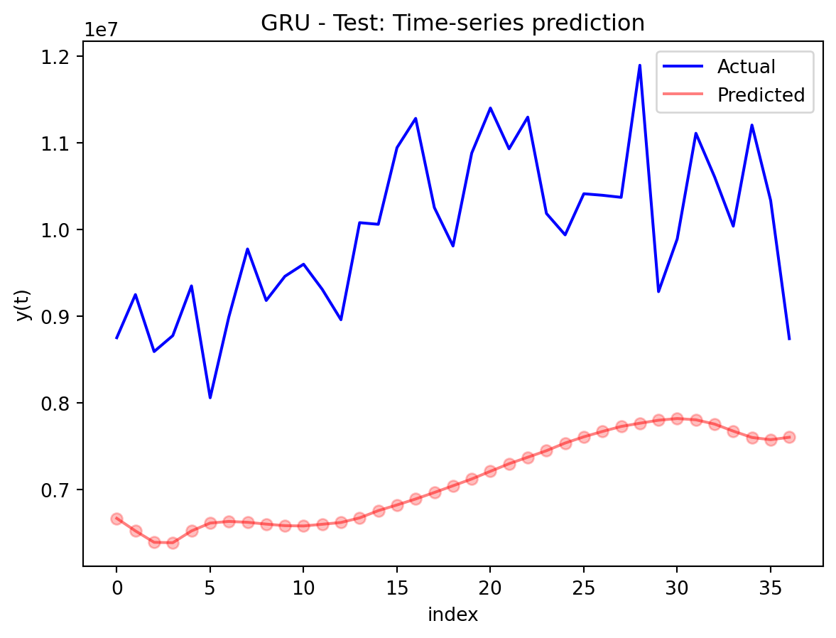
In the multivariate setting with South Korea’s exports to the U.S., the GRU is clearly the strongest of the three deep models, the LSTM is in the middle, and the plain RNN performs worst. The GRU achieves the lowest test RMSE and MAE, and its forecast line tracks the held-out test data more closely than the others, with relatively tight residuals and no obvious drift. The LSTM still manages to capture the upward trend but with noticeably larger errors and more volatility around turning points. The RNN, by contrast, has much higher errors and tends to indicate that a simple recurrent architecture struggles to summarize all the information in the multivariate input window. Overall, for this dataset the additional gating structure in the GRU seems genuinely useful, allowing it to exploit cross-series information and longer-range dependencies that the basic RNN cannot handle, while LSTM’s extra complexity does not translate into better accuracy given the data size.
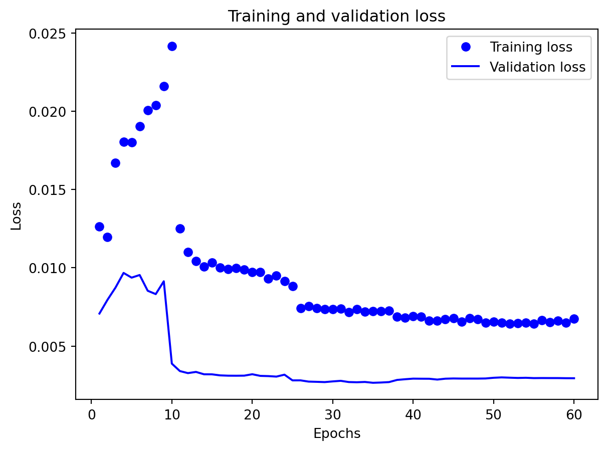
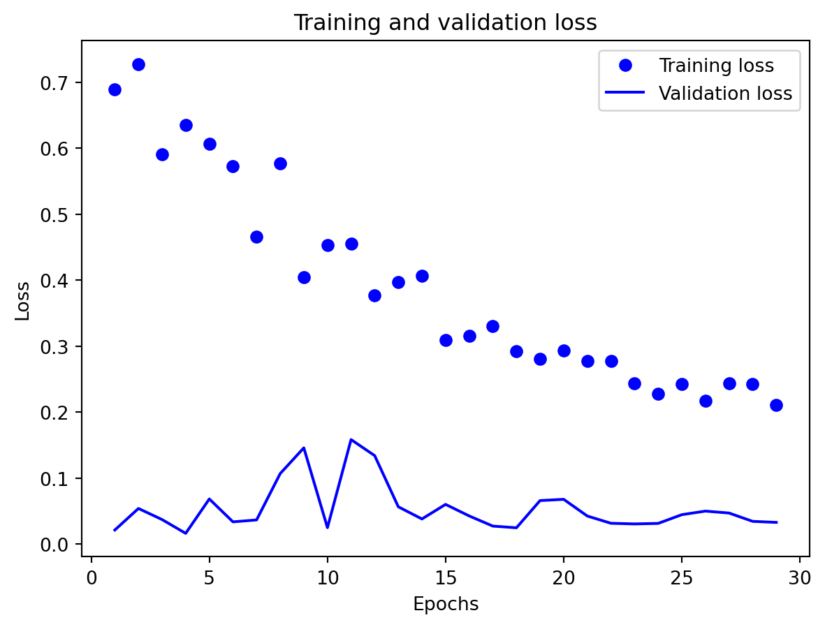
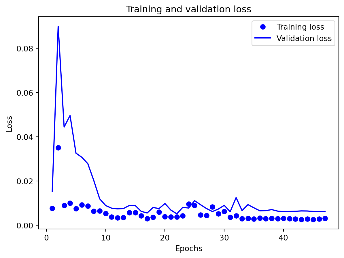
Effectiveness of regularization All three multivariate models share the same regularization,dropout on the recurrent stacks, early stopping on validation loss, and adaptive learning-rate reduction—and this setup performed well on preventing catastrophic overfitting even for the relatively large GRU and LSTM. Training and validation losses stay reasonably close to each other, and early stopping consistently triggers before the maximum epoch budget is used, which suggests that the models are not simply memorizing the training portion of the export series. Still, the gap in performance between GRU, LSTM, and especially RNN shows that regularization alone cannot rescue a poorly matched architecture: the RNN remains underpowered for the multivariate dynamics, and the LSTM appears somewhat over-parameterized. Concluding, regularization stabilizes learning and improves generalization somewhat, but choosing an appropriate architecture (here, the GRU) matters more than further tuning dropout or patience settings.
Comparison with SARIMAX (traditional multivariate model) Compared with the traditional model, the traditional model still has the edge: SARIMAX achieves a substantially lower test RMSE than any of the recurrent networks, while also producing stable, interpretable dynamics. This indicates that much of the structure in the export series—trend, seasonality, and relatively simple lag relationships—is well captured by linear time-series methods once you allow for appropriate differencing and seasonal terms. The GRU comes closest but still cannot match SARIMAX’s accuracy, and it requires more tuning effort and offers far less transparency about how shocks propagate through time. Taken together, the evidence suggests that for this particular multivariate macro dataset, SARIMAX is the most effective workhorse model, with the GRU being a reasonable nonlinear alternative.RNN and LSTM, however, appear dominated by these two in both performance and practicality.
Forecasting & Final model summary
Code
comparison_exports = pd.DataFrame({'Model': ['RNN', 'LSTM', 'GRU'],'Test RMSE': [results_exports_rnn['test_rmse'], results_exports_lstm['test_rmse'], results_exports_gru['test_rmse']],'Train Time (s)': [results_exports_rnn['train_time'], results_exports_lstm['train_time'], results_exports_gru['train_time']]})best_exports = comparison_exports.loc[comparison_exports['Test RMSE'].idxmin(), 'Model']print(f"\nBest model (South Korea Exports): {best_exports}")if best_exports =='RNN': forecast_exports = generate_forecast( results_exports_rnn['model'], results_exports_rnn['X_test'], results_exports_rnn['scalers'], n_steps=30 ) best_results = results_exports_rnnelif best_exports =='LSTM': forecast_exports = generate_forecast( results_exports_lstm['model'], results_exports_lstm['X_test'], results_exports_lstm['scalers'], n_steps=30 ) best_results = results_exports_lstmelse: forecast_exports = generate_forecast( results_exports_gru['model'], results_exports_gru['X_test'], results_exports_gru['scalers'], n_steps=30 ) best_results = results_exports_gruprint("\n"+"="*60)print("South Korea EXPORTS TO USA - FINAL COMPARISON")print("="*60)print(comparison_exports.to_string(index=False))fig = plot_forecast_exports_plotly( results_dict=best_results, best_model_name=best_exports, forecast_orig=forecast_exports, df4=df4, lookback=LOOKBACK, confidence=0.95)
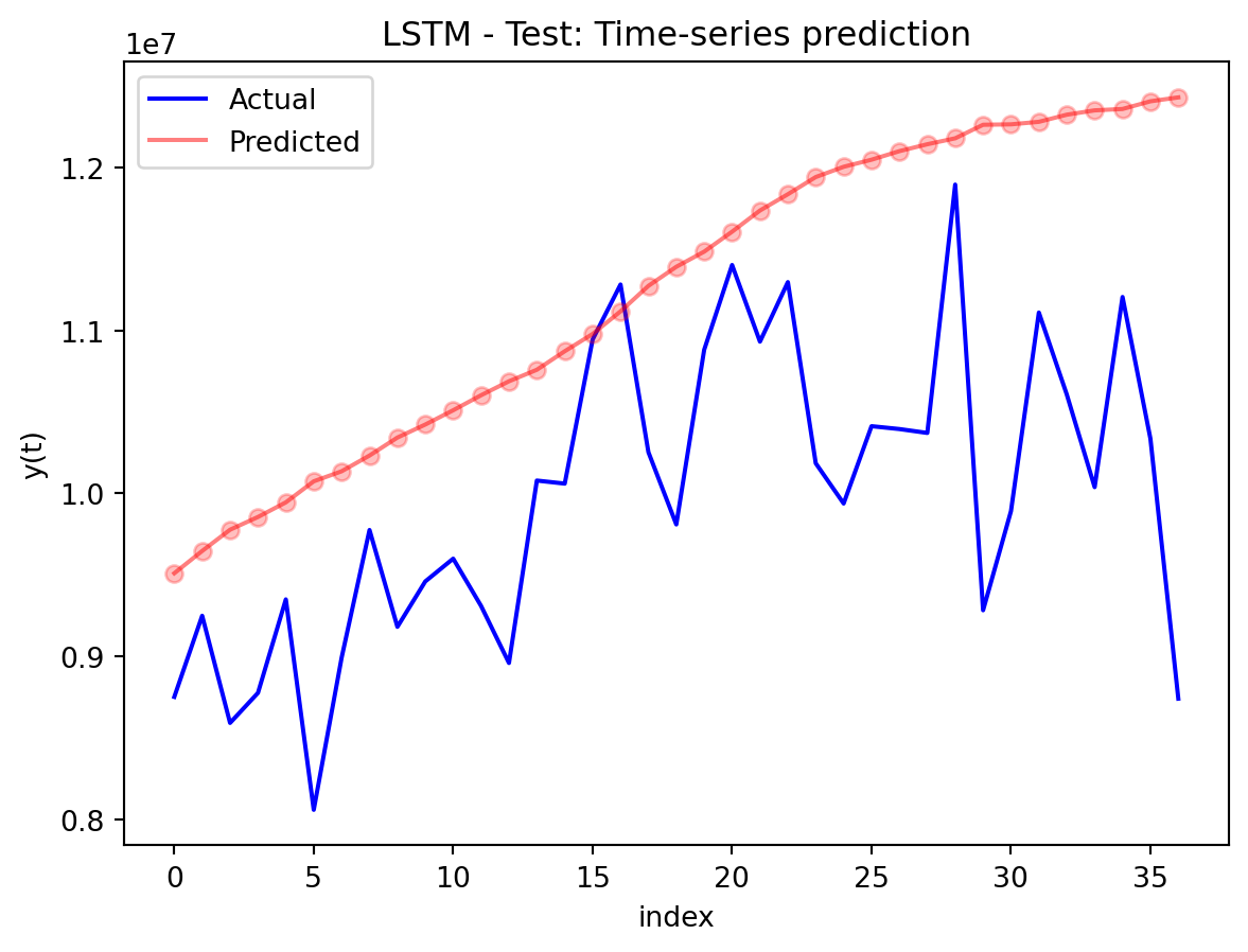
Best model (South Korea Exports): LSTM
Generating 30-step forecast...

============================================================
South Korea EXPORTS TO USA - FINAL COMPARISON
============================================================
Model    Test RMSE  Train Time (s)
  RNN 2.745355e+06        4.853161
 LSTM 1.493633e+06       15.459108
  GRU 2.976324e+06        9.018401
Forecast horizon and behavior
For the exports example, the best model forward is to produce a 12-month forecast, which reveals how these networks behave as the horizon extends. The GRU’s forecast starts near the last observed value and then follows a smooth, almost monotonic upward path, with an empirically based 95% confidence band that gradually widens the further you move from the forecast origin. Over the first few steps, the model’s predictions look quite plausible as short-term continuations of the recent trend, but as you approach the end of the year-ahead window, the forecasts become increasingly dominated by an extrapolated trend rather than detailed seasonal or cyclical structure—local fluctuations that appear in the historical data are largely smoothed away. This pattern suggests that the multivariate GRU is most reliable for short-to-medium horizons (a few months ahead), where it is still anchored by recent observations; deeper into the 12-month horizon, its output is better interpreted as a trend scenario with quantified uncertainty than as a precise monthly prediction.